Cube object

MPDAF Cube objects contain a series of images at neighboring wavelengths. These are stored as a 3D array of pixel values. The wavelengths of the images increase along the first dimension of this array, while the Y and X axes of the images lie along the second and third dimensions. In addition to the data array, Cubes contain a WaveCoord object that describes the wavelength scale of the spectral axis of the cube, and a WCS object that describes the spatial coordinates of the spatial axes. Optionally a 3D array of variances can be provided to give the statistical uncertainties of the fluxes. Finally a mask array is provided for indicating bad pixels.

The fluxes and their variances are stored in numpy masked arrays, so virtually all numpy and scipy functions can be applied to them.

Preliminary imports:

In [1]: import numpy as np

In [2]: import matplotlib.pyplot as plt

In [3]: import astropy.units as u

In [4]: from mpdaf.obj import Cube, WCS, WaveCoord

Cube creation

There are two common ways to obtain a Cube object:

• A cube can be created from a user-provided 3D array of pixel values, or from both a 3D array of pixel values, and a corresponding 3D array of variances. These can be simple numpy arrays, or they can be numpy masked arrays in which bad pixels have been masked. For example:

In [5]: wcs1 = WCS(crval=0, cdelt=0.2)

In [6]: wave1 = WaveCoord(cdelt=1.25, crval=4000.0, cunit=u.angstrom)

# numpy data array
In [7]: MyData = np.ones((400, 30, 30))

# cube filled with MyData
In [8]: cube = Cube(data=MyData, wcs=wcs1, wave=wave1) # cube 400X30x30 filled with data

In [9]: cube.info()
[INFO] 400 x 30 x 30 Cube (no name)
[INFO] .data(400 x 30 x 30) (no unit), no noise
[INFO] spatial coord (pix): min:(0.0,0.0) max:(5.8,5.8) step:(0.2,0.2) rot:-0.0 deg
[INFO] wavelength: min:4000.00 max:4498.75 step:1.25 Angstrom

• Alternatively, a cube can be read from a FITS file. In this case the flux and variance values are read from specific extensions:

# data and variance arrays read from the file (extension DATA and STAT)
In [10]: obj1 = Cube('../data/obj/CUBE.fits')

In [11]: obj1.info()
[INFO] 1595 x 10 x 20 Cube (../data/obj/CUBE.fits)
[INFO] .data(1595 x 10 x 20) (1e-40 erg / (Angstrom cm2 s)), .var(1595 x 10 x 20)
[INFO] center:(-30:00:00.4494,01:20:00.4376) size in arcsec:(2.000,4.000) step in arcsec:(0.200,0.200) rot:-0.0 deg
[INFO] wavelength: min:7300.00 max:9292.50 step:1.25 Angstrom

By default, if a FITS file has more than one extension, then it is expected to have a ‘DATA’ extension that contains the pixel data, and possibly a ‘STAT’ extension that contains the corresponding variances. If the file doesn’t contain extensions of these names, the “ext=” keyword can be used to indicate the appropriate extension or extensions.

The spatial and spectral world-coordinates of a Cube are recorded within WCS and WaveCoord objects, respectively. When a cube is read from a FITS file, these are automatically generated, based on FITS header keywords. Alternatively, when an cube is extracted from another cube, they are derived from the world coordinate information of the original cube.

In the above example, information about a cube is printed using the info method. In this case the information is as follows:

• The cube has dimensions, 1595 x 10 x 20, which means that there are 1595 images of different wavelengths, each having 10 x 20 spatial pixels.
• In addition to the pixel array (.data(1595 x 10 x 20)), there is also a variance array of the same dimensions (.var(1595 x 10 x 20)).
• The flux units of the pixels are 10^-20 erg/s/cm²/Angstrom.
• The center of the field of view is at DEC: -30° 0’ 0.45” and RA: 1°20‘0.437”.
• The size of the field of view is 2 arcsec x 4 arcsec. The pixel dimensions are 0.2 arcsec x 0.2 arcsec.
• The rotation angle of the field is 0°, which means that North is along the positive Y axis.
• The wavelength range is 7300-9292.5 Angstrom with a step of 1.25 Angstrom

The indexing of the cube arrays follows the Python conventions for indexing a 3D array. The pixel in the bottom-lower-left corner is referenced as [0,0,0] and the pixel [k,p,q] refers to the horizontal position q, the vertical position p, and the spectral position k, as follows:

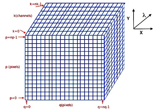
(see Spectrum, Image and Cube format for more information).

The following example computes a reconstructed white-light image and displays it. The white-light image is obtained by summing each spatial pixel of the cube along the wavelength axis. This converts the 3D cube into a 2D image. The cube in this examples contains an observation of a single galaxy.

In [12]: ima1 = obj1.sum(axis=0)

In [13]: plt.figure()
Out[13]: <matplotlib.figure.Figure at 0x7fb745ec9350>

In [14]: ima1.plot(scale='arcsinh', colorbar='v')
Out[14]: <matplotlib.image.AxesImage at 0x7fb745af2e90>

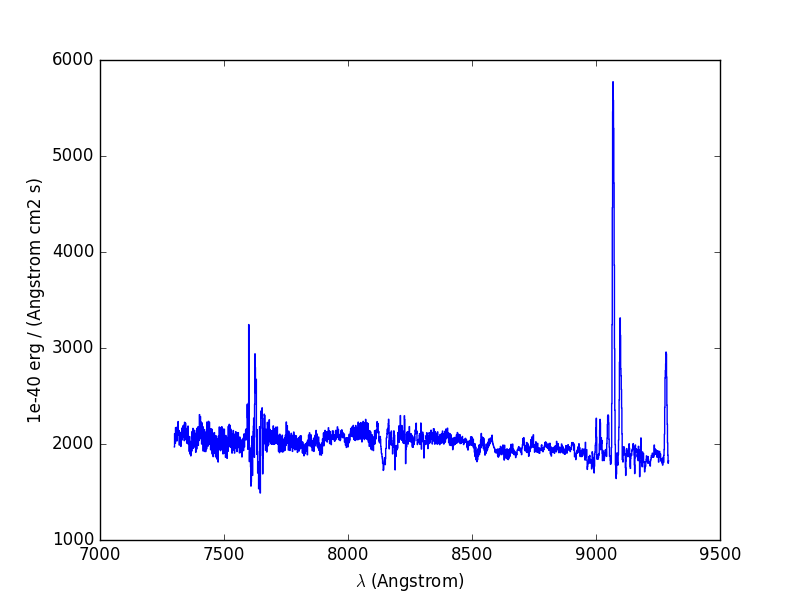
The next example computes the overall spectrum of the cube by taking the cube and summing along the X and Y axes of the image plane. This yields the total flux per spectral pixel.

In [15]: sp1 = obj1.sum(axis=(1,2))

In [16]: plt.figure()
Out[16]: <matplotlib.figure.Figure at 0x7fb748def110>

In [17]: sp1.plot()

Loops over all spectra

The examples in this section will demonstrate how a procedure can be applied iteratively to the spectra of every image pixel of a cube. The goal of the examples will be to create a version of the above data-cube that has had the continuum background subtracted. For each image pixel, a low-order polynomial will be fitted to the spectrum of that pixel. This results in a polynomial curve that approximates the continnum spectrum of the pixel. This polynomial is then subtracted from the spectrum of that pixel, and the difference spectrum is recorded in a new output cube.

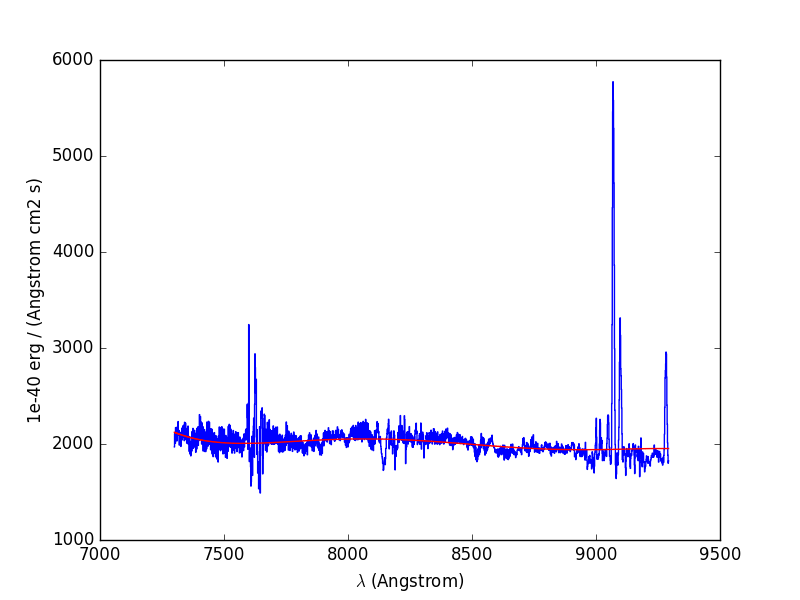
To illustrate the procedure, we start by fitting the continuum to the overal spectrum that was obtained in the previous example:

In [18]: plt.figure()
Out[18]: <matplotlib.figure.Figure at 0x7fb747e52f90>

In [19]: cont1 = sp1.poly_spec(5)

In [20]: sp1.plot()

In [21]: cont1.plot(color='r')

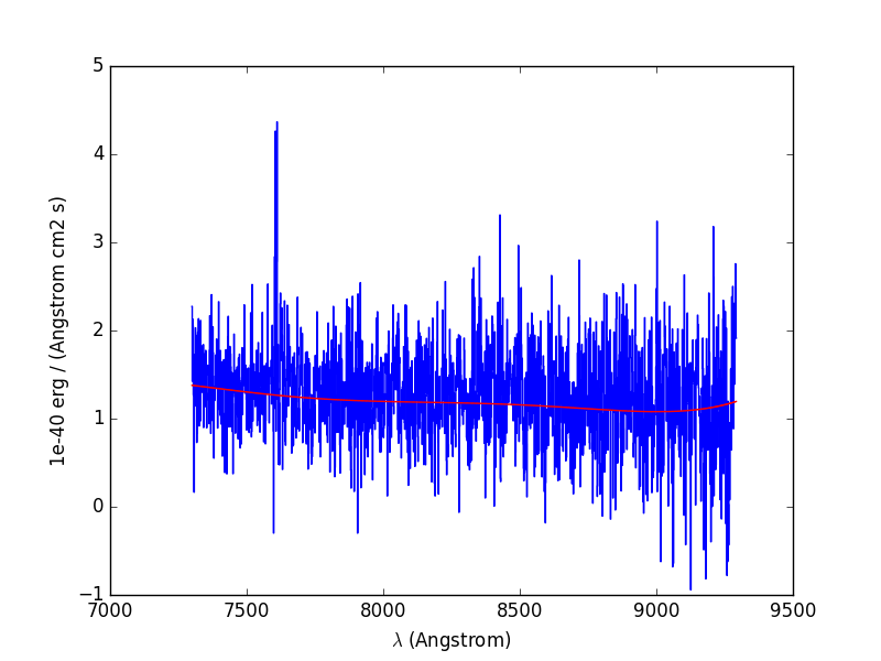
Next we do the same to a single pixel at the edge of the galaxy:

In [22]: plt.figure()
Out[22]: <matplotlib.figure.Figure at 0x7fb747adda90>

In [23]: sp1 = obj1[:,5,2]

In [24]: sp1.plot()

In [25]: sp1.poly_spec(5).plot(color='r')

In principle, the above procedure could be performed to each pixel by writing a nested loop over the X and Y axes of the cube. However, instead of using two loops, one can use the spectrum iterator method, iter_spe of the Cube object. In the following example this is used to iteratively extract the six spectra of a small 2 x 3 pixel sub-cube, and determine their peak values:

In [26]: from mpdaf.obj import iter_spe

In [27]: small = obj1[:,0:2,0:3]

In [28]: small.shape
Out[28]: (1595, 2, 3)

In [29]: for sp in iter_spe(small):
   ....:     print sp.data.max()
   ....: 

Now let’s use the same approach to do the continuum subtraction procedure. We start by creating an empty datacube with the same dimensions as the original cube, but without variance information (using the clone method). Using two spectrum iterators we iteratively extract the spectra of each image pixel of the input cube and the empty output cube. At each iteration we then fit a polynomial spectrum to the input spectrum and record it in the output spectrum.

In [30]: cont1 = obj1.clone(data_init=np.empty, var_init=np.zeros)

In [31]: for sp, co in zip(iter_spe(obj1), iter_spe(cont1)):
   ....:     co[:] = sp.poly_spec(5)
   ....: 

The result is a continuum datacube. Note that we have used the co[:] = sp.poly_spec(5) assignment rather than the more intuitive co = sp.poly_spec(5) assignment. The difference is that in python co=value changes the object that the co variable refers to, whereas co[:] changes the contents of the object that it currently points to. We want to change the contents of the spectrum in the output cube, so the latter is needed.

There is another way to compute the continuum datacube that can be much faster when used on a computer with multiple processors. This is to use the loop_spe_multiprocessing function. This uses multiple processors to apply a specified function to each spectrum of a cube and return a new cube that contains the resulting spectra:

In [32]: from mpdaf.obj import Spectrum

In [33]: cont2 = obj1.loop_spe_multiprocessing(f=Spectrum.poly_spec, deg=5)
[INFO] loop_spe_multiprocessing (poly_spec): 200 tasks

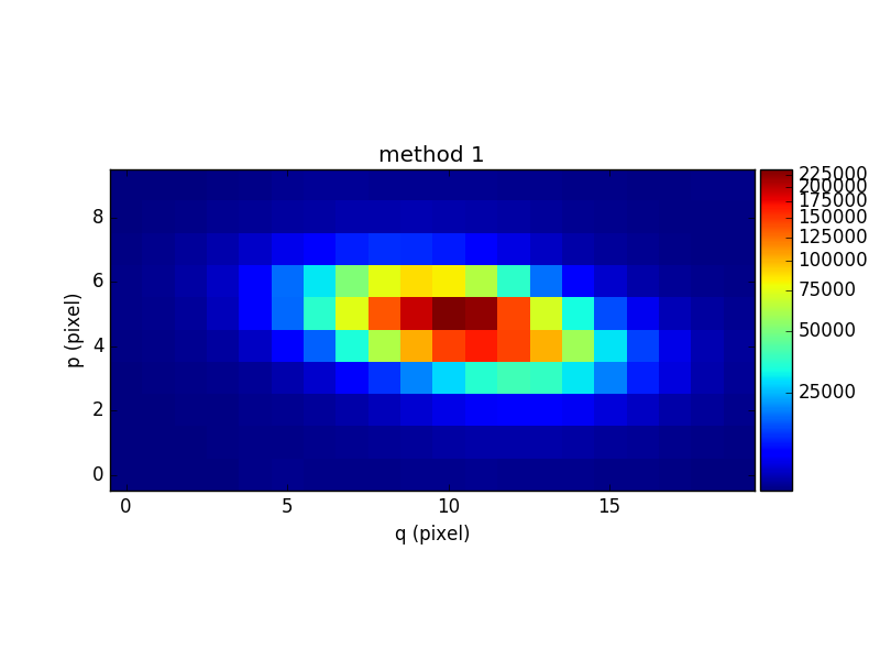
To compare the results of the two methods, the following example sums the images of the two continuum cubes over the wavelength axis and displays the resulting white-light images of the continuum:

In [34]: rec1 = cont1.sum(axis=0)

In [35]: plt.figure()
Out[35]: <matplotlib.figure.Figure at 0x7fb74449f950>

In [36]: rec1.plot(scale='arcsinh', colorbar='v', title='method 1')
Out[36]: <matplotlib.image.AxesImage at 0x7fb737c05b90>

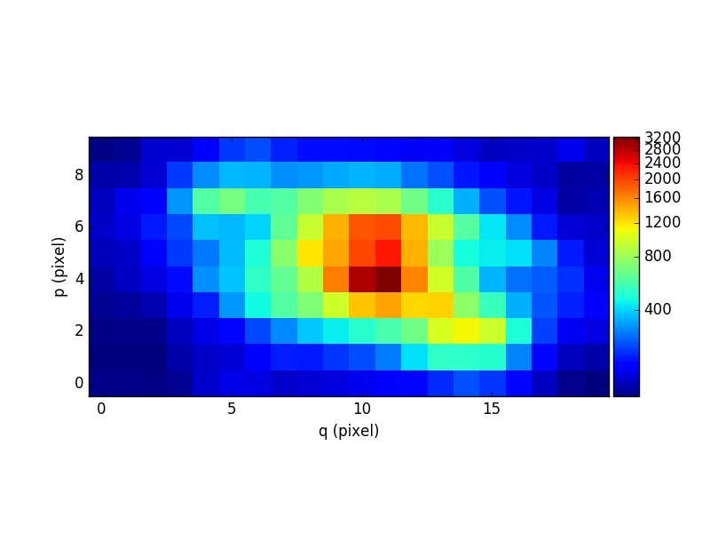
In [37]: rec2 = cont2.sum(axis=0)

In [38]: plt.figure()
Out[38]: <matplotlib.figure.Figure at 0x7fb74449c210>

In [39]: rec2.plot(scale='arcsinh', colorbar='v', title='method2')
Out[39]: <matplotlib.image.AxesImage at 0x7fb737c5abd0>

Next we subtract the continuum cube from the original cube to obtain a cube of the line emission of the galaxy. For display purposes this is then summed along the wavelength axis to yield an image of the sum of all of the emission lines in the cube:

In [40]: line1 = obj1 - cont1

In [41]: plt.figure()
Out[41]: <matplotlib.figure.Figure at 0x7fb745340fd0>

In [42]: line1.sum(axis=0).plot(scale='arcsinh', colorbar='v')
Out[42]: <matplotlib.image.AxesImage at 0x7fb7442f7fd0>

Next we compute the equivalent width of the Hα emission in the galaxy. First we isolate the emission line by truncating the object datacube in wavelength:

In [43]: plt.figure()
Out[43]: <matplotlib.figure.Figure at 0x7fb744335490>

# Obtain the overall spectrum of the cube.
In [44]: sp1 = obj1.sum(axis=(1,2))

In [45]: sp1.plot()

# Obtain the spectral pixel indexes of wavelengths 9000 and 9200
In [46]: k1,k2 = sp1.wave.pixel([9000,9200], nearest=True)

# Extract a sub-cube restricted to the above range of wavelengths.
In [47]: emi1 = obj1[k1:k2+1,:,:]

In [48]: emi1.info()
[INFO] 161 x 10 x 20 Cube (../data/obj/CUBE.fits)
[INFO] .data(161 x 10 x 20) (1e-40 erg / (Angstrom cm2 s)), .var(161 x 10 x 20)
[INFO] center:(-30:00:00.4494,01:20:00.4376) size in arcsec:(2.000,4.000) step in arcsec:(0.200,0.200) rot:-0.0 deg
[INFO] wavelength: min:9000.00 max:9200.00 step:1.25 Angstrom

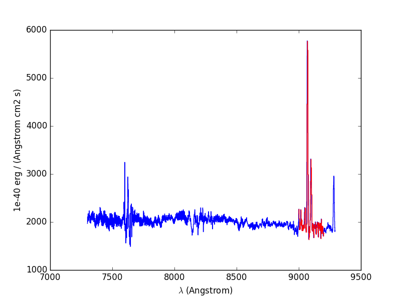
# Obtain the overall spectrum of the above sub-cube.
In [49]: sp1 = emi1.sum(axis=(1,2))

# Plot the sub-spectrum in red over the original spectrum.
In [50]: sp1.plot(color='r')

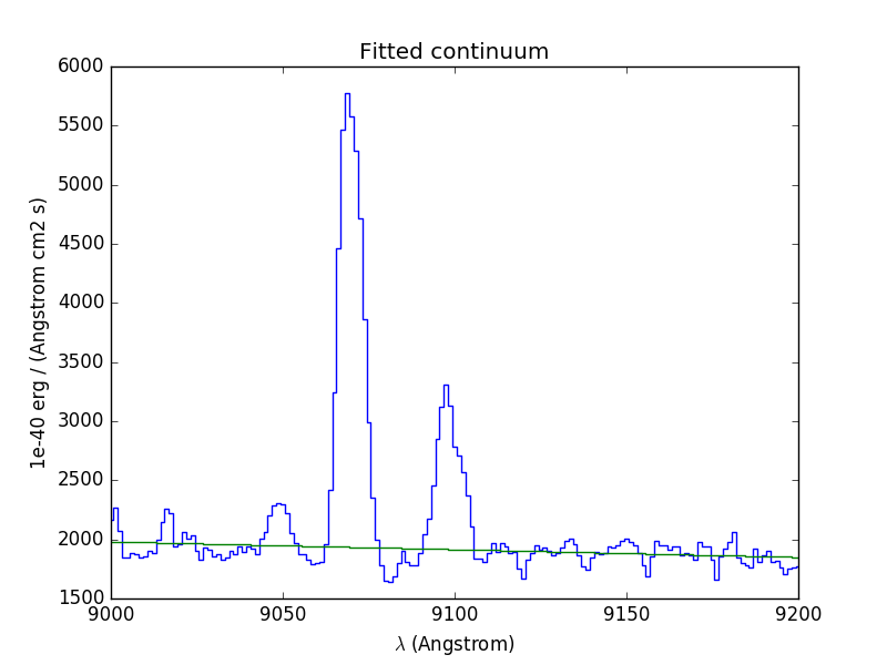
Next we fit and subtract the continuum. Before doing the polynomial fit we mask the region of the emission lines (sp1.mask), so that the lines don’t affect the fit, and then we perform a linear fit between the continuum on either side of the masked region. Then the spectrum is unmasked and the continuum subtracted:

In [51]: plt.figure()
Out[51]: <matplotlib.figure.Figure at 0x7fb737d75690>

# Mask the region containing the line emission.
In [52]: sp1.mask_region(9050, 9125)

# Fit a line to the continuum on either side of the masked region.
In [53]: cont1 = sp1.poly_spec(1)

# Unmask the region containing the line emission.
In [54]: sp1.unmask()

In [55]: plt.figure()
Out[55]: <matplotlib.figure.Figure at 0x7fb744396950>

In [56]: sp1.plot()

In [57]: cont1.plot(title="Fitted continuum")

In [58]: plt.figure()
Out[58]: <matplotlib.figure.Figure at 0x7fb74410af10>

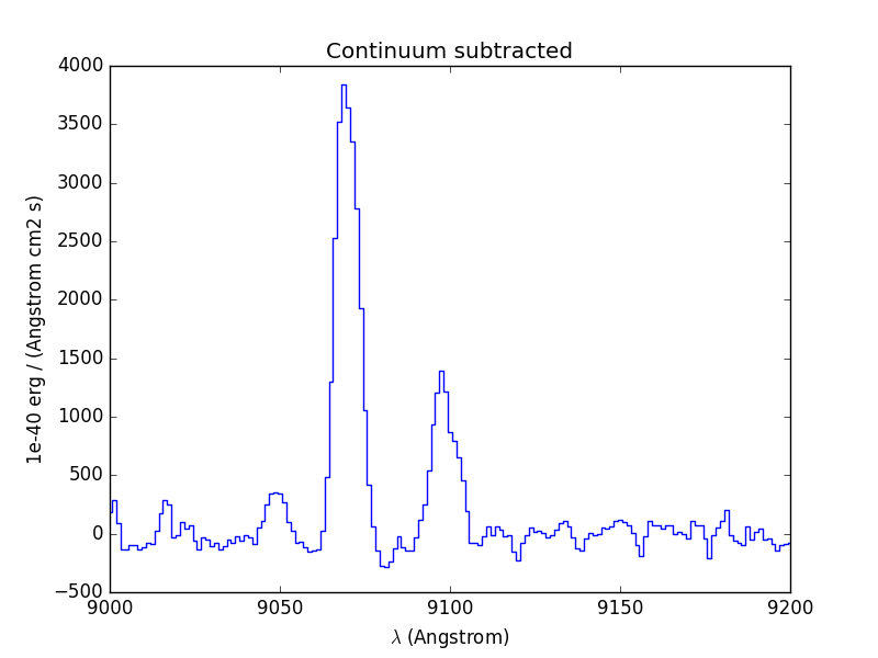
# Subtract the continuum from the spectrum to leave the line emission.
In [59]: line1 = sp1 - cont1

In [60]: line1.plot(title="Continuum subtracted")

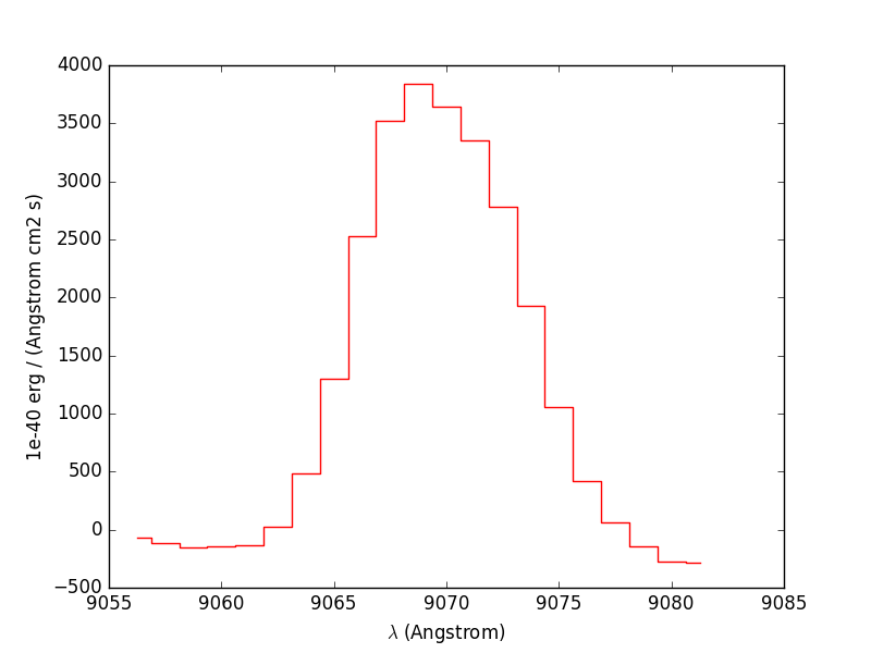
Next we compute the total Hα line flux by simple integration (taking into account the pixel size in Angstrom) over the wavelength range centered around the Hα line and the continuum mean flux at the same location:

In [61]: plt.figure()
Out[61]: <matplotlib.figure.Figure at 0x7fb737fef310>

# Find the spectral pixel index of the peak flux.
In [62]: k = line1.data.argmax()

In [63]: line1[55-10:55+11].plot(color='r')

# Integrate by summing pixels, multiplied by the pixel width.
In [64]: fline = (line1[55-10:55+11].sum()*line1.unit) * (line1.get_step(unit=line1.wave.unit)*line1.wave.unit)

# Obtain the mean continuum flux.
In [65]: cline = cont1[55-10:55+11].mean()*cont1.unit

# Compute the equivalent width of the line.
In [66]: ew = fline/cline

In [67]: print fline, cline, ew
9224.61872579 1e-40 erg / (cm2 s) 1936.55733796 1e-40 erg / (Angstrom cm2 s) 4.76341110329 Angstrom

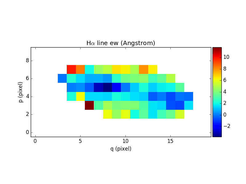
Finally we repeat this for all datacube spectra, and we save the Hα flux and equivalent width in two images. We start by creating two images with identical shapes and world-coordinates for the reconstructed image and then use the spectrum iterator iter_spe:

In [68]: ha_flux = ima1.clone(data_init=np.empty)

In [69]: cont_flux = ima1.clone(data_init=np.empty)

In [70]: ha_ew = ima1.clone(data_init=np.empty)

In [71]: for sp,pos in iter_spe(emi1, index=True):
   ....:     p,q = pos
   ....:     sp.mask_region(9050, 9125)
   ....:     cont = sp.poly_spec(1)
   ....:     sp.unmask()
   ....:     line = sp - cont
   ....:     fline = line[55-10:55+11].sum() * line.get_step(unit=line.wave.unit)
   ....:     cline = cont[55-10:55+11].mean()
   ....:     ew = fline/cline
   ....:     cont_flux[p,q] = cline
   ....:     ha_flux[p,q] = fline
   ....:     ha_ew[p,q] = ew
   ....: 

In [72]: plt.figure()
Out[72]: <matplotlib.figure.Figure at 0x7fb737ee46d0>

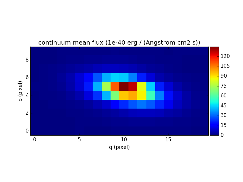
In [73]: cont_flux.plot(title="continuum mean flux (%s)"%cont_flux.unit, colorbar='v')
Out[73]: <matplotlib.image.AxesImage at 0x7fb737e63dd0>

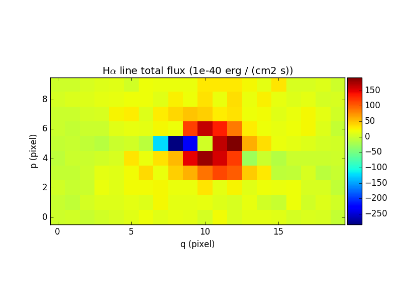
In [74]: ha_flux.unit = sp.unit * sp.wave.unit

In [75]: plt.figure()
Out[75]: <matplotlib.figure.Figure at 0x7fb737ee4690>

In [76]: ha_flux.plot(title="H$\\alpha$ line total flux (%s)"%ha_flux.unit, colorbar='v')
Out[76]: <matplotlib.image.AxesImage at 0x7fb7363a9bd0>

In [77]: ha_ew.mask_selection(np.where((ima1.data)<4000))

In [78]: ha_ew.unit = ha_flux.unit / cont_flux.unit

In [79]: plt.figure()
Out[79]: <matplotlib.figure.Figure at 0x7fb737db0bd0>

In [80]: ha_ew.plot(title="H$\\alpha$ line ew (%s)"%ha_ew.unit, colorbar='v')
Out[80]: <matplotlib.image.AxesImage at 0x7fb7362acf90>

Loops over all images

In this section, we demonstrate ways to perform of procedure iteratively to each image of a cube. We consider the datacube as a collection of monochromatic images and we process each of them. For each monochromatic image we apply a convolution by a gaussian kernel.

# Data and variance arrays read from the file (extension DATA and STAT)
In [81]: cube = Cube('../data/obj/Central_Datacube_bkg.fits')

First, we use the image iterator iter_ima, which operates similarly to the spectrum iterator described earlier on this page, except that it returns successive images instead of successive spectra:

In [82]: from mpdaf.obj import iter_ima

In [83]: cube2 = cube.clone(data_init=np.empty, var_init=np.empty)

In [84]: for ima,k in iter_ima(cube, index=True):
   ....:     cube2[k,:,:] = ima.gaussian_filter(sigma=3)
   ....: 

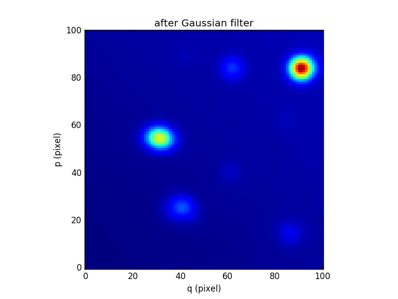
We can also make use of multiple processors to do the same thing faster, by using the loop_ima_multiprocessing method. This applies a specified procedure to all images within a cube and returns a new cube of the processed images:

In [85]: from mpdaf.obj import Image

In [86]: cube2 = cube.loop_ima_multiprocessing(f=Image.gaussian_filter, sigma=3)

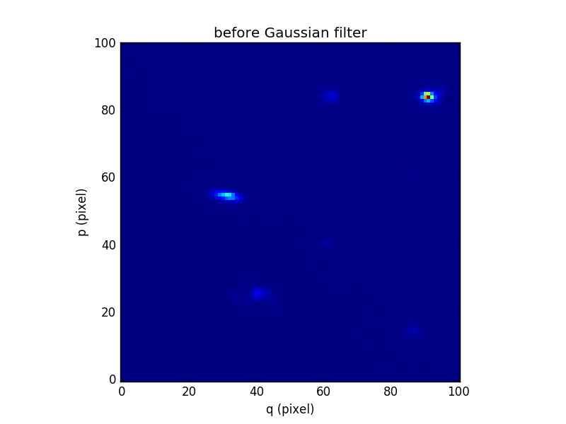
We then plot the results:

In [87]: plt.figure()
Out[87]: <matplotlib.figure.Figure at 0x7fb73618d350>

In [88]: cube.sum(axis=0).plot(title='before Gaussian filter')
Out[88]: <matplotlib.image.AxesImage at 0x7fb735fec150>

In [89]: plt.figure()
Out[89]: <matplotlib.figure.Figure at 0x7fb73621d350>

In [90]: cube2.sum(axis=0).plot(title='after Gaussian filter')
Out[90]: <matplotlib.image.AxesImage at 0x7fb735f11dd0>

Next we will use the loop_ima_multiprocessing method to fit and remove a background gradient from a simulated datacube. For each image of the cube, we fit a 2nd order polynomial to the background values (selected here by simply applying a flux threshold to mask all bright objects). We do so by doing a chi^2 minimization over the polynomial coefficients using the numpy recipe np.linalg.lstsq(). For this, we define a function that takes an image as its sole parameter and returns a background-subtracted image:

In [91]: def remove_background_gradient(ima):
   ....:     ksel = np.where(ima.data.data<2.5)
   ....:     pval = ksel[0]
   ....:     qval = ksel[1]
   ....:     zval = ima.data.data[ksel]
   ....:     degree = 2
   ....:     Ap = np.vander(pval,degree)
   ....:     Aq = np.vander(qval,degree)
   ....:     A = np.hstack((Ap,Aq))
   ....:     (coeffs,residuals,rank,sing_vals) = np.linalg.lstsq(A,zval)
   ....:     fp = np.poly1d(coeffs[0:degree])
   ....:     fq = np.poly1d(coeffs[degree:2*degree])
   ....:     X,Y = np.meshgrid(range(ima.shape[0]), range(ima.shape[1]))
   ....:     ima2 = ima - np.array(map(lambda q,p: fp(p)+fq(q),Y,X))
   ....:     return ima2
   ....: 

We can then create the background-subtracted cube:

In [92]: cube2 = cube.loop_ima_multiprocessing(f=remove_background_gradient)

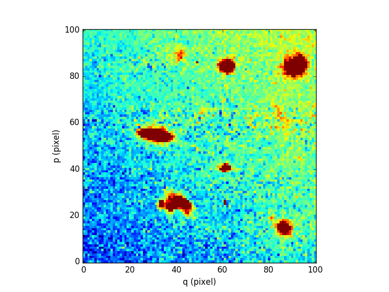
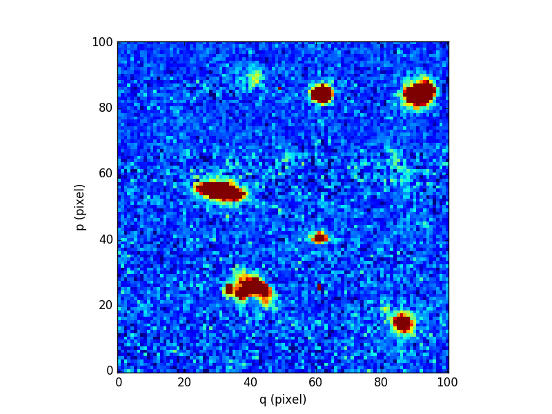
Finally, we compare the results for one of the slices:

In [93]: plt.figure()
Out[93]: <matplotlib.figure.Figure at 0x7fb735eebd10>

In [94]: cube[5,:,:].plot(vmin=-1, vmax=4)
Out[94]: <matplotlib.image.AxesImage at 0x7fb735e68d10>

In [95]: plt.figure()
Out[95]: <matplotlib.figure.Figure at 0x7fb735e1cf50>

In [96]: cube2[5,:,:].plot(vmin=-1, vmax=4)
Out[96]: <matplotlib.image.AxesImage at 0x7fb735db8890>

Sub-cube extraction

Warning

To be written.

mpdaf.obj.Cube.select_lambda returns the sub-cube corresponding to a wavelength range.

mpdaf.obj.Cube.get_image extracts an image around a position in the datacube.

mpdaf.obj.Cube.bandpass_image sums the images of a cube after multiplying the cube by the spectral bandpass curve of another instrument.

mpdaf.obj.Cube.subcube extracts a sub-cube around a position.

mpdaf.obj.Cube.aperture

mpdaf.obj.Cube.subcube_circle_aperture extracts a sub-cube from an circle aperture of fixed radius.