Getting Started
Importing MPDAF
MPDAF is divided into sub-packages, each of which is composed of several
classes. The following example shows how to import the Cube and
PixTable classes:
In [1]: from mpdaf.obj import Cube

In [2]: from mpdaf.drs import PixTable
All of the examples in the MPDAF web pages are shown being typed into
an interactive IPython shell. This shell is the origin of the prompts
like In [1]: in the above example. The examples can also be entered
in other shells, such as the native Python shell.
Loading your first MUSE datacube
MUSE datacubes are generally loaded from FITS files. In these files the fluxes and variances are stored in separate FITS extensions. For example:
# data and variance arrays are read from DATA and STAT extensions of the file
In [3]: cube = Cube('obj/CUBE.fits')

In [4]: cube.info()
[INFO] 1595 x 10 x 20 Cube (obj/CUBE.fits)
[INFO] .data(1595 x 10 x 20) (1e-40 erg / (Angstrom cm2 s)), .var(1595 x 10 x 20)
[INFO] center:(-30:00:00.4494,01:20:00.4376) size:(2.000",4.000") step:(0.200",0.200") rot:-0.0 deg frame:FK5
[INFO] wavelength: min:7300.00 max:9292.50 step:1.25 Angstrom
The listed dimensions of the cube, 1595 x 10 x 20, indicate that the cube has 1595 spectral pixels and 10 x 20 spatial pixels. The order in which these dimensions are listed, follows the indexing conventions used by Python to handle 3D arrays (see Spectrum, Image and Cube format for more information).
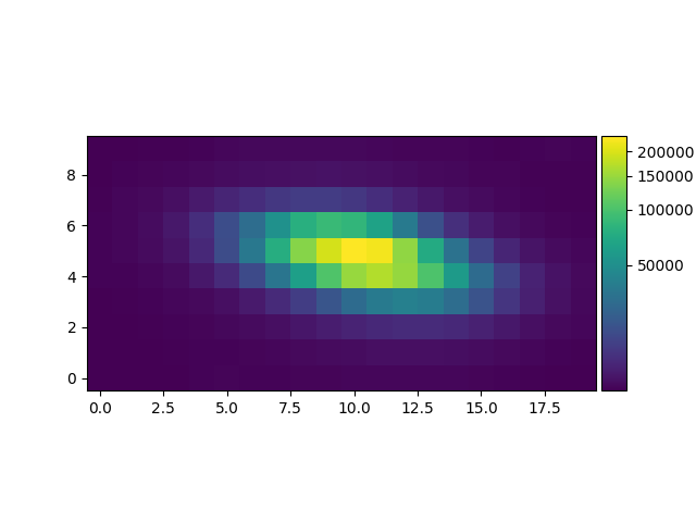
Let’s compute the reconstructed white-light image and display it. The white-light image is obtained by summing each spatial pixel of the cube along the wavelength axis. This converts the 3D cube into a 2D image.
In [5]: ima = cube.sum(axis=0)
In [6]: type(ima)
Out[6]: mpdaf.obj.image.Image
In [7]: plt.figure()
������������������������������Out[7]: <Figure size 640x480 with 0 Axes>
In [8]: ima.plot(scale='arcsinh', colorbar='v')
������������������������������������������������������������������������Out[8]: <matplotlib.image.AxesImage at 0x7fc7573f4710>
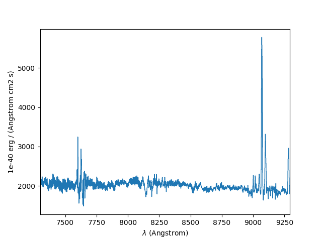
Let’s now compute the overall spectrum of the cube by taking the cube and summing along the X and Y axes of the image plane. This yields the total flux per spectral pixel.
In [9]: sp = cube.sum(axis=(1,2))
In [10]: type(sp)
Out[10]: mpdaf.obj.spectrum.Spectrum
In [11]: plt.figure()
�������������������������������������Out[11]: <Figure size 640x480 with 0 Axes>
In [12]: sp.plot()
Logging
When imported, MPDAF initialize a logger by default. This logger uses the
logging module, and log messages to stderr, for instance for the .info()
methods. See Logging (mpdaf.log) for more details.
Online Help
Because different sub-packages have very different functionality,
further suggestions for getting started are provided in the online
documentation of these sub-packages. For example, click on Cube object,
Image object, or Spectrum object for help with the 3 main classes of
the mpdaf.obj package.
Alternatively, if you use the IPython interactive python shell, then you can
look at the docstrings of classes, objects and functions by following them with
the magic ? of IPython. Examples of this are shown below. A more general
way to see these docstrings, which works in all Python shells, is to use the
built-in help() function:
In [13]: Cube.median?
Signature: Cube.median(self, axis=None)
Docstring:
Return the median over a given axis.

Beware that if the pixels of the cube have associated variances, these
are discarded by this function, because there is no way to estimate the
effects of a median on the variance.

Parameters
----------
axis : int or tuple of int, optional
    The axis or axes along which a median is performed.

    The default (axis = None) performs a median over all the
    dimensions of the cube and returns a float.

    axis = 0 performs a median over the wavelength dimension and
    returns an image.

    axis = (1,2) performs a median over the (X,Y) axes and
    returns a spectrum.
File:      ~/checkouts/readthedocs.org/user_builds/mpdaf/envs/3.2/lib/python3.6/site-packages/mpdaf/obj/cube.py
Type:      function
In [14]: help(ima.plot)
Help on method plot in module mpdaf.obj.image:

plot(title=None, scale='linear', vmin=None, vmax=None, zscale=False, colorbar=None, var=False, show_xlabel=False, show_ylabel=False, ax=None, unit=Unit("deg"), use_wcs=False, **kwargs) method of mpdaf.obj.image.Image instance
    Plot the image with axes labeled in pixels.

    If either axis has just one pixel, plot a line instead of an image.

    Colors are assigned to each pixel value as follows. First each
    pixel value, ``pv``, is normalized over the range ``vmin`` to ``vmax``,
    to have a value ``nv``, that goes from 0 to 1, as follows::

        nv = (pv - vmin) / (vmax - vmin)

    This value is then mapped to another number between 0 and 1 which
    determines a position along the colorbar, and thus the color to give
    the displayed pixel. The mapping from normalized values to colorbar
    position, color, can be chosen using the scale argument, from the
    following options:

    - 'linear': ``color = nv``
    - 'log': ``color = log(1000 * nv + 1) / log(1000 + 1)``
    - 'sqrt': ``color = sqrt(nv)``
    - 'arcsinh': ``color = arcsinh(10*nv) / arcsinh(10.0)``

    A colorbar can optionally be drawn. If the colorbar argument is given
    the value 'h', then a colorbar is drawn horizontally, above the plot.
    If it is 'v', the colorbar is drawn vertically, to the right of the
    plot.

    By default the image is displayed in its own plot. Alternatively
    to make it a subplot of a larger figure, a suitable
    ``matplotlib.axes.Axes`` object can be passed via the ``ax`` argument.
    Note that unless matplotlib interative mode has previously been enabled
    by calling ``matplotlib.pyplot.ion()``, the plot window will not appear
    until the next time that ``matplotlib.pyplot.show()`` is called. So to
    arrange that a new window appears as soon as ``Image.plot()`` is
    called, do the following before the first call to ``Image.plot()``::

        import matplotlib.pyplot as plt
        plt.ion()

    Parameters
    ----------
    title : str
        An optional title for the figure (None by default).
    scale : 'linear' | 'log' | 'sqrt' | 'arcsinh'
        The stretch function to use mapping pixel values to
        colors (The default is 'linear'). The pixel values are
        first normalized to range from 0 for values <= vmin,
        to 1 for values >= vmax, then the stretch algorithm maps
        these normalized values, nv, to a position p from 0 to 1
        along the colorbar, as follows:
        linear:  p = nv
        log:     p = log(1000 * nv + 1) / log(1000 + 1)
        sqrt:    p = sqrt(nv)
        arcsinh: p = arcsinh(10*nv) / arcsinh(10.0)
    vmin : float
        Pixels that have values <= vmin are given the color
        at the dark end of the color bar. Pixel values between
        vmin and vmax are given colors along the colorbar according
        to the mapping algorithm specified by the scale argument.
    vmax : float
        Pixels that have values >= vmax are given the color
        at the bright end of the color bar. If None, vmax is
        set to the maximum pixel value in the image.
    zscale : bool
        If True, vmin and vmax are automatically computed
        using the IRAF zscale algorithm.
    colorbar : str
        If 'h', a horizontal colorbar is drawn above the image.
        If 'v', a vertical colorbar is drawn to the right of the image.
        If None (the default), no colorbar is drawn.
    var : bool
          If true variance array is shown in place of data array
    ax : matplotlib.axes.Axes
        An optional Axes instance in which to draw the image,
        or None to have one created using ``matplotlib.pyplot.gca()``.
    unit : `astropy.units.Unit`
        The units to use for displaying world coordinates
        (degrees by default). In the interactive plot, when
        the mouse pointer is over a pixel in the image the
        coordinates of the pixel are shown using these units,
        along with the pixel value.
    use_wcs : bool
        If True, use `astropy.visualization.wcsaxes` to get axes
        with world coordinates.
    kwargs : matplotlib.artist.Artist
        Optional extra keyword/value arguments to be passed to
        the ``ax.imshow()`` function.

    Returns
    -------
    out : matplotlib AxesImage