MUSE specific tools (mpdaf.MUSE)

Python interface for MUSE slicer numbering scheme

The Slicer class contains a set of static methods to convert a slice number between the various numbering schemes. The definition of the various numbering schemes and the conversion table can be found in the “Global Positioning System” document (VLT-TRE-MUSE-14670-0657).

All the methods are static and thus there is no need to instantiate an object to use this class.

For example, we convert slice number 4 in CCD numbering to SKY numbering:

In [1]: from mpdaf.MUSE import Slicer

In [2]: Slicer.ccd2sky(4)
Out[2]: 10

Now we convert slice number 12 of stack 3 in OPTICAL numbering to CCD numbering:

In [3]: Slicer.optical2sky((2, 12))
Out[3]: 25

MUSE LSF models

Warning

LSF class is currently under development

Only one model of LSF (Line Spread Function) is currently available.

LSF qsim_v1

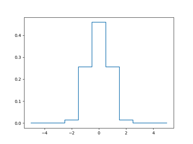
This is a simple model where the LSF is supposed to be constant over the filed of view. It uses a simple parametric model of variation with wavelength.

The model is a convolution of a step function with a Gaussian. The resulting function is then sample by the pixel size:

LSF = T(y2+dy/2) - T(y2-dy/2) - T(y1+dy/2) + T(y1-dy/2)

T(x) = exp(-x**2/2) + sqrt(2*pi)*x*erf(x/sqrt(2))/2

y1 = (y-h/2) / sigma

y2 = (y+h/2) / sigma

The slit width is assumed to be constant (h = 2.09 pixels). The Gaussian sigma parameter is a polynomial approximation of order 3 with wavelength:

c = [-0.09876662, 0.44410609, -0.03166038, 0.46285363]

sigma(x) = c[3] + c[2]*x + c[1]*x**2 + c[0]*x**3

To use it, create a LSF object with attribute ‘typ’ equal to ‘qsim_v1’:

In [4]: from mpdaf.MUSE import LSF

In [5]: lsf = LSF(typ='qsim_v1')

Then get the LSF array by using get_LSF:

In [6]: lsf_6000 = lsf.get_LSF(lbda=6000, step=1.25, size=11)

In [7]: import matplotlib.pyplot as plt

In [8]: import numpy as np

In [9]: plt.plot(np.arange(-5,6), lsf_6000, drawstyle='steps-mid')
Out[9]: [<matplotlib.lines.Line2D at 0x7f78462e8d68>]

MUSE FSF models

Warning

FSF class is currently under development

Two models of FSF (Field Spread Function) are currently available:

• OldMoffatModel (model='MOFFAT1'): the old model with a fixed beta.
• MoffatModel2 (model=2): a circular MOFFAT with polynomials for beta and FWHM.

Example with MOFFAT1

The MUSE FSF is supposed to be a Moffat function with a FWHM which varies linearly with the wavelength:

\(FWHM = a + b * lbda\)

With:

• beta (float) Power index of the Moffat.
• a (float) constant in arcsec which defined the FWHM.
• b (float) constant which defined the FWHM.

We create the FSFModel object like this:

In [10]: from mpdaf.MUSE import FSFModel, OldMoffatModel

In [11]: fsf = OldMoffatModel(a=0.885, b=-2.94E-05, beta=2.8, pixstep=0.2)

In [12]: isinstance(fsf, FSFModel)
Out[12]: True

Various methods allow to get the FSF array (2D or 3D, as mpdaf Image or Cube) for given wavelengths, or the FWHM in pixel and in arcseconds.

In [13]: lbda = np.array([5000, 9000])

In [14]: fsf.get_fwhm(lbda)
Out[14]: array([0.738 , 0.6204])

In [15]: fsf.get_fwhm(lbda, unit='pix')
Out[15]: array([3.69 , 3.102])

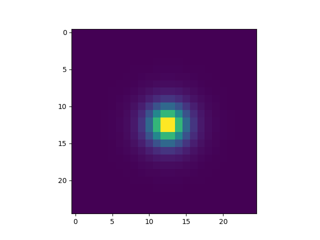
In [16]: im5000 = fsf.get_2darray(lbda[0], shape=(25, 25))

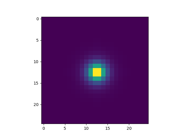
In [17]: fsfcube = fsf.get_3darray(lbda, shape=(25, 25))

In [18]: plt.figure()
Out[18]: <Figure size 640x480 with 0 Axes>

In [19]: plt.imshow(im5000)
Out[19]: <matplotlib.image.AxesImage at 0x7f7851691d30>

In [20]: plt.figure()
Out[20]: <Figure size 640x480 with 0 Axes>

In [21]: plt.imshow(fsfcube[1])
Out[21]: <matplotlib.image.AxesImage at 0x7f78511f2588>

The FSF model can be saved to a FITS header with mpdaf.MUSE.FSFModel.to_header, and read with mpdaf.MUSE.FSFModel.read.

MUSE mosaic field map

Warning

FieldsMap class is currently under development

FieldsMap reads the possible FIELDMAP extension of the MUSE data cube.

In [22]: from mpdaf.MUSE import FieldsMap

In [23]: fmap = FieldsMap('sdetect/subcub_mosaic.fits', extname='FIELDMAP')

get_pixel_fields returns a list of fields that cover a given pixel (y, x):

In [24]: fmap.get_pixel_fields(0,0)
Out[24]: ['UDF-06', 'UDF-09']

In [25]: fmap.get_pixel_fields(20,20)
Out[25]: ['UDF-06']

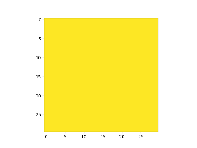
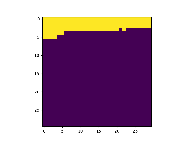
get_field_mask returns an array with non-zeros values for pixels matching a field:

In [26]: plt.figure()
Out[26]: <Figure size 640x480 with 0 Axes>

In [27]: plt.imshow(fmap.get_field_mask('UDF-06'), vmin=0, vmax=1)
Out[27]: <matplotlib.image.AxesImage at 0x7f78514aca58>

In [28]: plt.figure()
Out[28]: <Figure size 640x480 with 0 Axes>

In [29]: plt.imshow(fmap.get_field_mask('UDF-09'), vmin=0, vmax=1)
Out[29]: <matplotlib.image.AxesImage at 0x7f78514c8cc0>

Reference/API

mpdaf.MUSE Package

Functions

FSF([typ])	This class offers Field Spread Function (FSF) models for MUSE.
Moffat2D(fwhm, beta, shape[, center, normalize])	Compute Moffat for a value or array of values of FWHM and beta.
create_psf_cube(shape, fwhm[, beta, wcs, …])	Create a PSF cube with FWHM varying along each wavelength plane.
get_FSF_from_cube_keywords(cube, size)	Return a cube of FSFs corresponding to the keywords presents in the MUSE data cube primary header (‘FSF***’)

Classes

FSFModel()	Base class for FSF models.
FieldsMap([filename, nfields])	Class to work with the mosaic field map.
LSF([typ])	This class offers Line Spread Function models for MUSE.
MoffatModel2(fwhm_pol, beta_pol, lbrange, …)
OldMoffatModel(a, b, beta, pixstep[, field])	Moffat FSF with fixed beta and FWHM varying with wavelength.
Slicer	Convert slice number between the various numbering schemes.

Class Inheritance Diagram