Image object
Image objects contain a 2D data array of flux values, and a WCS object that describes the spatial coordinates of the
image. Optionally, an array of variances can also be provided to give the
statistical uncertainties of the fluxes. These can be used for weighting the
flux values and for computing the uncertainties of least-squares fits and other
calculations. Finally a mask array is provided for indicating bad pixels.
The fluxes and their variances are stored in numpy masked arrays, so virtually all numpy and scipy functions can be applied to them.
Preliminary imports:
In [1]: import numpy as np

In [2]: import matplotlib.pyplot as plt

In [3]: import astropy.units as u

In [4]: from mpdaf.obj import Image, WCS
Image creation
There are two common ways to obtain an Image object:
- An image can be created from a user-provided 2D array of the pixel values, or from both a 2D array of pixel values, and a corresponding 2D array of variances. These can be simple numpy arrays, or they can be numpy masked arrays in which bad pixels have been masked. For example:
In [5]: wcs1 = WCS(crval=0, cdelt=0.2)

# numpy data array
In [6]: MyData = np.ones((300,300))

# image filled with MyData
In [7]: ima = Image(data=MyData, wcs=wcs1) # image 300x300 filled with data

In [8]: ima.info()
[INFO] 300 x 300 Image (no name)
[INFO] .data(300 x 300) (no unit), no noise
[INFO] spatial coord (pix): min:(0.0,0.0) max:(59.8,59.8) step:(0.2,0.2) rot:-0.0 deg
- Alternatively, an image can be read from a FITS file. In this case the flux and variance values are read from specific extensions:
# data and variance arrays read from the file (extension DATA and STAT)
In [9]: ima = Image('obj/IMAGE-HDFS-1.34.fits')

In [10]: ima.info()
[INFO] 331 x 326 Image (obj/IMAGE-HDFS-1.34.fits)
[INFO] .data(331 x 326) (1e-20), .var(331 x 326)
[INFO] center:(-60:33:48.9321,22:32:55.5267) size:(66.200",65.200") step:(0.200",0.200") rot:-0.0 deg frame:ICRS
By default, if a FITS file has more than one extension, then it is expected to have a ‘DATA’ extension that contains the pixel data, and possibly a ‘STAT’ extension that contains the corresponding variances. If the file doesn’t contain extensions of these names, the “ext=” keyword can be used to indicate the appropriate extension or extensions.
The world-coordinate grid of an Image is described by a WCS
object. When an image is read from a FITS file, this is automatically generated
based on FITS header keywords. Alternatively, when an image is extracted from a
cube or another image, the WCS object is derived from the WCS object of the
original object.
As shown in the above example, information about an image can be printed using
the info method.
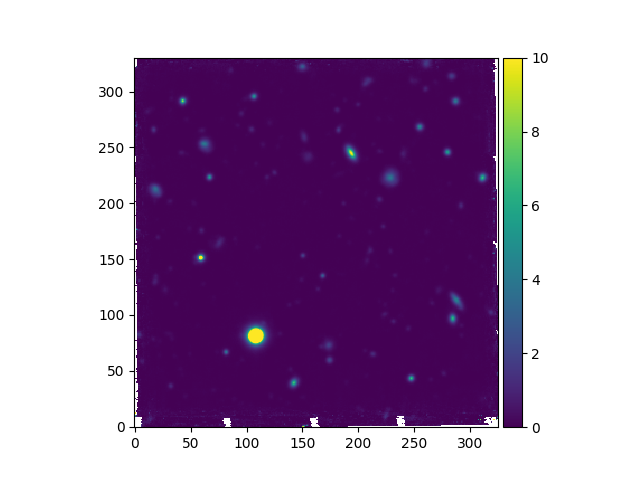
Image objects provide a plot method that is based on
matplotlib.pyplot.plot and
accepts all matplotlib arguments. The colors used to plot an image are
distributed between a minimum and a maximum pixel value. By default these are
the minimum and maximum pixel values in the image, but different thresholds can
be specified via the vmin and vmax arguments, as shown below.
In [11]: plt.figure()
Out[11]: <Figure size 640x480 with 0 Axes>
In [12]: ima.plot(vmin=0, vmax=10, colorbar='v')
�������������������������������������������Out[12]: <matplotlib.image.AxesImage at 0x7fc756d06710>
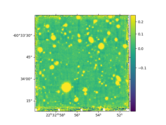
The plot method has many options to customize the plot, for
instance:
In [13]: plt.figure()
Out[13]: <Figure size 640x480 with 0 Axes>
In [14]: ima.plot(zscale=True, colorbar='v', use_wcs=True, scale='sqrt')
�������������������������������������������Out[14]: <matplotlib.image.AxesImage at 0x7fc7575f8c88>
The indexing of the image arrays follows the Python conventions for indexing a 2D array. For an MPDAF image im, the pixel in the lower-left corner is referenced as im[0,0] and the pixel im[p,q] refers to the horizontal pixel q and the vertical pixel p, as follows:
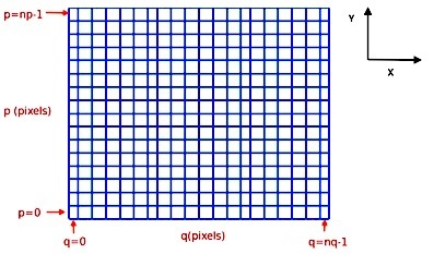
In total, this image im contains nq pixels in the horizontal direction and np pixels in the vertical direction (see Spectrum, Image and Cube format for more information).
Image Geometrical manipulation
In the following example, the sky is rotated within the image by 40 degrees anticlockwise, then re-sampled to change its pixel size from 0.2 arcseconds to 0.4 arcseconds.
In [15]: import astropy.units as u

In [16]: fig, (ax1, ax2, ax3) = plt.subplots(1, 3, figsize=(12, 4), tight_layout=True)

In [17]: ima.plot(ax=ax1, colorbar='v')
Out[17]: <matplotlib.image.AxesImage at 0x7fc7585a8780>

In [18]: ima2 = ima.rotate(40) #this rotation uses an interpolation of the pixels

In [19]: ima2.plot(ax=ax2, colorbar='v')
Out[19]: <matplotlib.image.AxesImage at 0x7fc75918a978>

In [20]: ima3 = ima2.resample(newdim=(150,150), newstart=None, newstep=(0.4,0.4), unit_step=u.arcsec, flux=True)

In [21]: ima3.plot(ax=ax3, colorbar='v')
Out[21]: <matplotlib.image.AxesImage at 0x7fc7574cfc18>
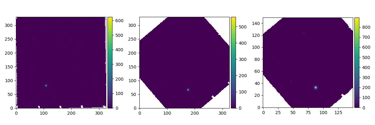
The rotate method interpolates the image onto a
rotated coordinate grid.
The resample method also interpolates the image
onto a new grid, but before doing this it applies a decimation filter to remove
high spatial frequencies that would otherwise be undersampled by the pixel
spacing.
The newstart=None argument indicates that the sky position that appears at
the center of pixel [0,0] should also be at the center of pixel [0,0] of the
resampled image. This argument can alternatively be used to move the sky within
the image.
The resample method is a simplified interface to
the regrid function, which provides more options.
The following example shows how images from different telescopes can be resampled onto the same coordinate grid, then how the coordinate offsets of the pixels can be adjusted to account for relative pointing errors:
# Read a small part of an HST image
In [22]: imahst = Image('obj/HST-HDFS.fits')
# Resample the HST image onto the coordinate grid of the MUSE image
In [23]: ima2hst = imahst.align_with_image(ima)
In [24]: plt.figure()
Out[24]: <Figure size 640x480 with 0 Axes>
In [25]: ima.plot(colorbar='v', vmin=0.0, vmax=20.0, title='MUSE image')
�������������������������������������������Out[25]: <matplotlib.image.AxesImage at 0x7fc757d8f828>
In [26]: plt.figure()
Out[26]: <Figure size 640x480 with 0 Axes>
In [27]: ima2hst.plot(colorbar='v', title='Part of the HST image')
�������������������������������������������Out[27]: <matplotlib.image.AxesImage at 0x7fc757064898>
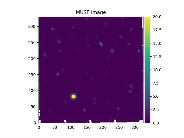
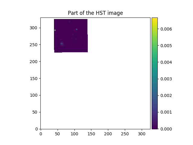
In the example shown above, the align_with_image method resamples an HST image onto the same
coordinate grid as a MUSE image. The resampled HST image then has the same
number of pixels, and the same pixel coordinates as the MUSE image.
The adjust_coordinates method then uses
an enhanced form of cross-correlation to estimate and correct for any relative
pointing errors between the two images. Note that, to see the estimated
correction without applying it, the estimate_coordinate_offset method could have been used.
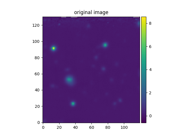
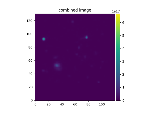
In the following example, the aligned HST and MUSE images are combined to produce a higher S/N image. Note the use of the addition operator to add the two images:
In [28]: ima2hst[ima2hst.mask] = 0
In [29]: ima2hst.unmask()
In [30]: imacomb = ima + ima2hst
In [31]: plt.figure()
Out[31]: <Figure size 640x480 with 0 Axes>
In [32]: ima[200:, 30:150].plot(colorbar='v', title='original image')
�������������������������������������������Out[32]: <matplotlib.image.AxesImage at 0x7fc756d4e438>
In [33]: plt.figure()
Out[33]: <Figure size 640x480 with 0 Axes>
In [34]: imacomb[200:, 30:150].plot(colorbar='v', title='combined image')
�������������������������������������������Out[34]: <matplotlib.image.AxesImage at 0x7fc756b1a7f0>
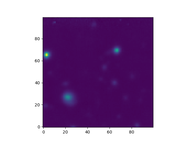
The subimage method can be used to extract a square
or rectangular sub-image of given world-coordinate dimensions from an image. In
the following example it is used used to extract a 20 arcsecond square sub-image
from the center of the HST image.
In [35]: dec, ra = imahst.wcs.pix2sky(np.array(imahst.shape)/2)[0]
In [36]: subima = ima.subimage(center=(dec,ra), size=20.0)
In [37]: plt.figure()
Out[37]: <Figure size 640x480 with 0 Axes>
In [38]: subima.plot()
�������������������������������������������Out[38]: <matplotlib.image.AxesImage at 0x7fc7566c56a0>
The inside method lets the user test whether a given
coordinate is inside an image. In the following example, dec and ra are the
coordinates of the center of the image that were calculated in the preceding
example.
In [39]: subima.inside([dec, ra])
Out[39]: True
In [40]: subima.inside(ima.get_start())
��������������Out[40]: False
Object analysis: image segmentation, peak measurement, profile fitting
The following demonstration will show some examples of extracting and analyzing
images of individual objects within an image. The first example segments the
image into several cutout images using the (segment)
method:
In [41]: im = Image('obj/a370II.fits')

In [42]: seg = im.segment(minsize=10, background=2100)
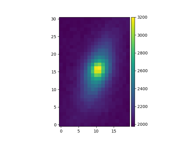
The segment method returns a list of images of the
detected sources. In the following example, we extract one of these for further
analysis:
In [43]: source = seg[8]
In [44]: plt.figure()
Out[44]: <Figure size 640x480 with 0 Axes>
In [45]: source.plot(colorbar='v')
�������������������������������������������Out[45]: <matplotlib.image.AxesImage at 0x7fc74f091ef0>
For a first approximation, some simple analysis methods are applied:
backgroundto estimate the background level,peakto locate the peak of the source,fwhmto estimate the FWHM of the source.
# background value and its standard deviation
In [46]: source.background()
Out[46]: (2052.505415162455, 68.01699304230651)
# peak position and intensity
In [47]: source.peak()
������������������������������������������������Out[47]:
{'x': 40.02632730206195,
'y': -1.6018629119499264,
'p': 15.880560309635259,
'q': 10.834926649327759,
'data': 3201}
# fwhm in arcsec
In [48]: source.fwhm()
���������������������������������������������������������������������������������������������������������������������������������������������������������������������������������Out[48]: array([0.67815839, 0.63540917])
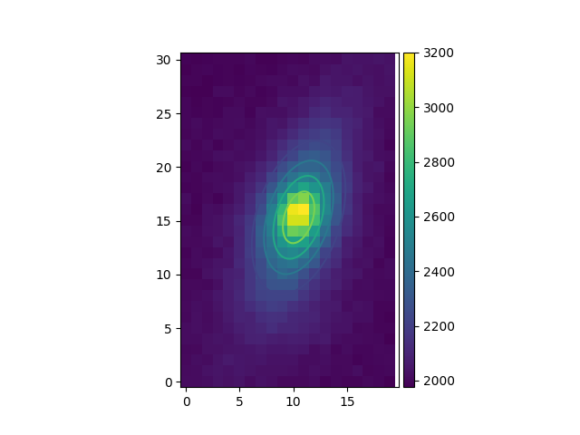
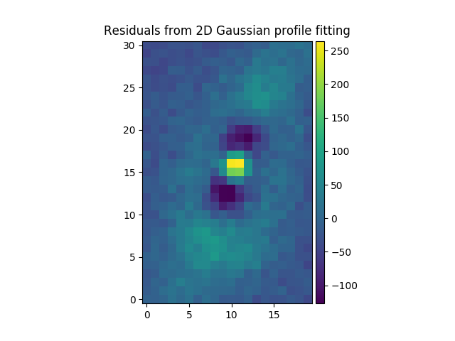
Then, for greater accuracy we fit a 2D Gaussian to the source, and plot the
isocontours (gauss_fit):
In [49]: gfit = source.gauss_fit(plot=False)
[INFO] Gaussian center = (-1.60183,40.0263) (error:(2.40391e-06,1.46758e-06))
[INFO] Gaussian integrated flux = 51445.8 (error:687.259)
[INFO] Gaussian peak value = 940.004 (error:-8.98435)
[INFO] Gaussian fwhm = (1.96076,1.04189) (error:(0.0224652,0.0119394))
[INFO] Rotation in degree: 162.395 (error:1.41177)
[INFO] Gaussian continuum = 2022.39 (error:1.86548)
In [50]: gfit = source.gauss_fit(maxiter=150, plot=True)
����������������������������������������������������������������������������������������������������������������������������������������������������������������������������������������������������������������������������������������������������������������������������������������������������������������������������������������������������������������������������[INFO] Gaussian center = (-1.60183,40.0263) (error:(2.40391e-06,1.46758e-06))
[INFO] Gaussian integrated flux = 51445.8 (error:687.259)
[INFO] Gaussian peak value = 940.004 (error:-8.98435)
[INFO] Gaussian fwhm = (1.96076,1.04189) (error:(0.0224652,0.0119394))
[INFO] Rotation in degree: 162.395 (error:1.41177)
[INFO] Gaussian continuum = 2022.39 (error:1.86548)
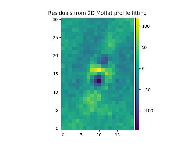
In general, Moffat profiles provide a better representation of the point-spread
functions of ground-based telescope observations, so next we perform a 2D MOFFAT
fit to the same source (moffat_fit):
In [51]: mfit = source.moffat_fit(plot=True)
[INFO] center = (-1.60183,40.0263) (error:(1.46452e-06,8.9727e-07))
[INFO] integrated flux = 253370 (error:0.000110584)
[INFO] peak value = 1217.37 (error:15.1703)
[INFO] fwhm = (1.56078,0.832519) (error:(0.0196986,0.986155))
[INFO] n = 1.13844 (error:0.0514963)
[INFO] rotation in degree: 162.373 (error:0.453644)
[INFO] continuum = 1964.35 (error:4.31709)
We then subtract the fitted Gaussian and Moffat models of from the original
source to see the residuals. Note the use of gauss_image and
moffat_image to create MPDAF images of the 2D Gaussian and Moffat
functions:
In [52]: from mpdaf.obj import gauss_image, moffat_image
In [53]: gfitim = gauss_image(wcs=source.wcs, gauss=gfit)
In [54]: mfitim = moffat_image(wcs=source.wcs, moffat=mfit)
In [55]: gresiduals = source-gfitim
In [56]: mresiduals = source-mfitim
In [57]: plt.figure()
Out[57]: <Figure size 640x480 with 0 Axes>
In [58]: mresiduals.plot(colorbar='v', title='Residuals from 2D Moffat profile fitting')
�������������������������������������������Out[58]: <matplotlib.image.AxesImage at 0x7fc74ed75f60>
In [59]: plt.figure()
Out[59]: <Figure size 640x480 with 0 Axes>
In [60]: gresiduals.plot(colorbar='v', title='Residuals from 2D Gaussian profile fitting')
�������������������������������������������Out[60]: <matplotlib.image.AxesImage at 0x7fc74ed0f3c8>
Finally we estimate the energy received from the source:
- The
eemethod computes ensquared or encircled energy, which is the sum of the flux within a given radius of the center of the source.- The
ee_sizemethod computes the size of a square centered on the source that contains a given fraction of the total flux of the source,- The
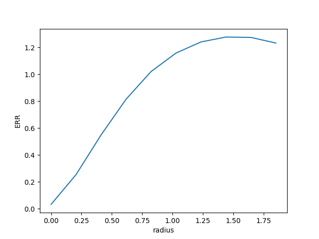
eer_curvemethod returns the normalized enclosed energy as a function radius.
# Obtain the encircled flux within a radius of one FWHM of the source
In [61]: source.ee(radius=source.fwhm(), cont=source.background()[0])
Out[61]: 32765.64259927794
# Get the enclosed energy normalized by the total energy as a function of radius (ERR)
In [62]: radius, ee = source.eer_curve(cont=source.background()[0])
# The size of the square centered on the source that contains 90% of the energy (in arcsec)
In [63]: source.ee_size()
Out[63]: array([4.26351015, 4.26816953])
In [64]: plt.figure()
�����������������������������������������Out[64]: <Figure size 640x480 with 0 Axes>
In [65]: plt.plot(radius, ee)
������������������������������������������������������������������������������������Out[65]: [<matplotlib.lines.Line2D at 0x7fc74ec460b8>]
In [66]: plt.xlabel('radius')
�������������������������������������������������������������������������������������������������������������������������������������������Out[66]: Text(0.5, 0, 'radius')
In [67]: plt.ylabel('ERR')
���������������������������������������������������������������������������������������������������������������������������������������������������������������������������Out[67]: Text(0, 0.5, 'ERR')