Source object
A lot of tools are currently been developed to detect sources in MUSE data
cubes. In order to easily exchange information about detected sources, we
needed to define a format for storing source file. A FITS file format has been
defined and is described in the Source ICD.
The Source class implements input/output for this Source FITS file and methods
to analyse, plot and compare source objects.
Warning
Source class is currently under development
A Source object O consist of:
Component |
Description |
|---|---|
O.header |
pyfits header instance |
O.lines |
astropy table that contains the parameters of spectral lines. |
O.z |
astropy table that contains redshift values. |
O.mag |
astropy table that contains magnitude values. |
O.spectra |
Dictionary that contains spectra.
Keys give description of the spectra.
Values are |
O.images |
Dictionary that contains images.
Keys gives filter names.
Values are |
O.cubes |
Dictionary that contains small data cubes.
Keys give description of the cubes.
Values are |
O.tables |
Dictionary that contains astropy tables. Keys give description of the tables. Values are astropy table objects. |
Create a source
First, we create a source object from spatial coordinates (by using from_data):
In [1]: from mpdaf.sdetect import Source

In [2]: s = Source.from_data(ID=36, ra=338.2260, dec=-60.5640, origin=('test','v0.0','DATACUBE-HDFS.fits', 'v1.34'))
info print information:
In [3]: s.info()
[INFO] ID      =                   36 / object ID %d
[INFO] RA      =              338.226 / RA u.degree %.7f
[INFO] DEC     =              -60.564 / DEC u.degree %.7f
[INFO] FROM    = 'test    '           / detection software
[INFO] FROM_V  = 'v0.0    '           / version of the detection software
[INFO] CUBE    = 'DATACUBE-HDFS.fits' / datacube
[INFO] CUBE_V  = 'v1.34   '           / version of the datacube
[INFO] SRC_V   = ''
[INFO] 0 spectra:
[INFO] 0 images:
[INFO] 0 cubes:
[INFO] 0 tables:
Information have been saved in the pyfits header instance but we can access and update each of them as an attribute:
In [4]: s.FROM
Out[4]: 'test'

In [5]: s.FROM = 'test2'
It is easy to add a new information that will be save as keyword in the FITS header. For example we save the pixel coordinates:
In [6]: from mpdaf.obj import Cube

In [7]: cube = Cube('DATACUBE-HDFS-1.34.fits')

In [8]: s.y, s.x = cube.wcs.sky2pix((s.dec,s.ra))[0]
Nevertheless, the special methods add_comment and add_history are recommended to save comment and history with the good syntax.
Now, we use the method add_cube to extract and save in the Source object a subcube of 5 arcseconds centered on the source center and for the 5000:8500 Angstroem range:
In [9]: s.add_cube(cube, 'MUSE', size=5, lbda=(5000,8500))
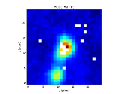
add_white_image method computes from the MUSE data cube a white image of 5 arcseconds around the object and appends it to the images dictionary:
In [10]: s.add_white_image(cube=cube, size=5)

In [11]: s.images['MUSE_WHITE'].plot(title='MUSE_WHITE')
Out[11]: <matplotlib.image.AxesImage at 0x7f66cdcee590>
add_image extracts an image centered on the source center and appends it to the images dictionary.
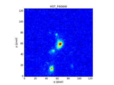
We can for example extract an HST image centered on the source center and append it to the images dictionary:
In [12]: from mpdaf.obj import Image

In [13]: ima_hst = Image('f606_comb.fits')

In [14]: s.add_image(ima_hst, name='HST_F606W')
If the parameter size is not present, the size of the image is by default the same as the white image (in arcsec).
In the same way:
add_narrow_band_imagescreates narrow band images from a redshift value and a catalog of lines.
add_narrow_band_image_lbdaobscreates a narrow band image around an observed wavelength value.
At the end our Source looks like that:
In [15]: s.info()
[INFO] FROM    = 'test2   '           / detection software
[INFO] CUBE    = 'DATACUBE-HDFS.fits' / MUSE data cube
[INFO] RA      =              338.226 / RA u.degree %.7f
[INFO] FROM  _V= 'v0.0    '           / version of the detection software
[INFO] Y       =    157.6590537314896
[INFO] X       =     209.926327090741
[INFO] DEC     =              -60.564 / DEC u.degree %.7f
[INFO] ID      =                   36 / object ID u.unitless %d

[INFO] images['HST_F606W'], 125 X 125 .data  rot=-0.5 deg
[INFO] images['MUSE_WHITE'], 25 X 25 .data .var rot=-0.0 deg
[INFO] cubes['MUSE'], 2801 X 25 X 25 .data .var rot=-0.0 deg
We can now write the Source object in a FITS file and load it latter by using from_file:
In [16]: s.write('source%04d.fits'%s.id)
Extract spectra
In this part, we will runs sextractor on the narrow-band images to define spectrum extraction apertures. This algorithm has been developed by Jarle Brinchmann (University of Leiden) and ported to python as the following methods:
add_seg_images runs SExtractor to create segmentation maps,
find_sky_mask creates a sky mask from the list of segmentation maps,
find_union_mask creates an object mask as the union of the segmentation maps,
find_intersection_mask creates an object mask as the intersection of the segmentation maps,
extract_spectra computes spectra from the MUSE data cube as the sum of the subcube weighted by different masks of the object.
Add lines and estimate the best redshift
add_line adds a line to the lines table.
sort_lines sorts the lines by flux in descending order.
crack_z estimates the best redshift matching the list of emission lines.
add_z adds a redshift value to the z table.
add_mag adds a magnitude value to the mag table.
SourceList class
SourceList is a sub-class of the python list class. This class contains just
one method mpdaf.sdetect.SourceList.write that creates a folder and saves all sources
files and the catalog file in it.