MUSE specific tools (mpdaf.MUSE)
Python interface for MUSE slicer numbering scheme
The Slicer class contains a set of static methods to convert
a slice number between the various numbering schemes. The definition of the
various numbering schemes and the conversion table can be found in the “Global
Positioning System” document (VLT-TRE-MUSE-14670-0657).
All the methods are static and thus there is no need to instantiate an object to use this class.
For example, we convert slice number 4 in CCD numbering to SKY numbering:
In [1]: from mpdaf.MUSE import Slicer

In [2]: Slicer.ccd2sky(4)
Out[2]: 10
Now we convert slice number 12 of stack 3 in OPTICAL numbering to CCD numbering:
In [3]: Slicer.optical2sky((2, 12))
Out[3]: 25
MUSE LSF models
Warning
LSF class is currently under development
Only one model of LSF (Line Spread Function) is currently available.
LSF qsim_v1
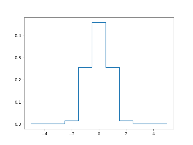
This is a simple model where the LSF is supposed to be constant over the filed of view. It uses a simple parametric model of variation with wavelength.
The model is a convolution of a step function with a Gaussian. The resulting function is then sample by the pixel size:
LSF = T(y2+dy/2) - T(y2-dy/2) - T(y1+dy/2) + T(y1-dy/2)

T(x) = exp(-x**2/2) + sqrt(2*pi)*x*erf(x/sqrt(2))/2

y1 = (y-h/2) / sigma

y2 = (y+h/2) / sigma
The slit width is assumed to be constant (h = 2.09 pixels). The Gaussian sigma parameter is a polynomial approximation of order 3 with wavelength:
c = [-0.09876662, 0.44410609, -0.03166038, 0.46285363]

sigma(x) = c[3] + c[2]*x + c[1]*x**2 + c[0]*x**3
To use it, create a LSF object with attribute ‘typ’ equal to
‘qsim_v1’:
In [4]: from mpdaf.MUSE import LSF

In [5]: lsf = LSF(typ='qsim_v1')
Then get the LSF array by using get_LSF:
In [6]: lsf_6000 = lsf.get_LSF(lbda=6000, step=1.25, size=11)

In [7]: import matplotlib.pyplot as plt

In [8]: import numpy as np

In [9]: plt.plot(np.arange(-5,6), lsf_6000, drawstyle='steps-mid')
Out[9]: [<matplotlib.lines.Line2D at 0x7f1063a3b780>]
MUSE FSF models
Warning
FSF class is currently under development
Only one model of FSF (Field Spread Function) is currently available.
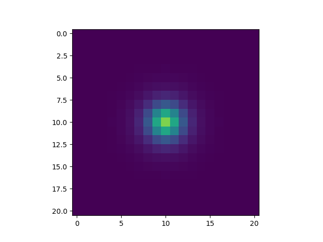
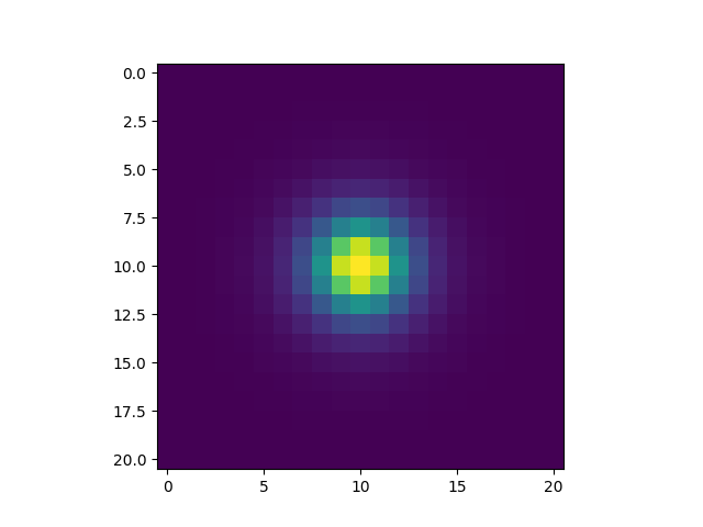
FSF MOFFAT1
The MUSE FSF is supposed to be a Moffat function with a FWHM which varies linearly with the wavelength:
fwhm = a + b*lbda
With:
- beta (float) Power index of the Moffat.
- a (float) constant in arcsec which defined the FWHM.
- b (float) constant which defined the FWHM.
We create the FSF object like this:
In [10]: from mpdaf.MUSE import FSF

In [11]: fsf = FSF(typ='MOFFAT1')
get_FSF returns for each wavelength an array and the FWHM in
pixel and in arcseconds.
In [12]: fsf_array, fwhm_pix, fwhm_arcsec = fsf.get_FSF(lbda=[5000, 9000], step=0.2, size=21, beta=2.8, a=0.885, b=-2.94E-05)
In [13]: print(fwhm_pix)
[3.69 3.102]
In [14]: print(fwhm_arcsec)
��������������[0.738 0.6204]
In [15]: plt.figure()
������������������������������Out[15]: <Figure size 640x480 with 0 Axes>
In [16]: plt.imshow(fsf_array[1], vmin=0, vmax=60, interpolation='nearest')
�������������������������������������������������������������������������Out[16]: <matplotlib.image.AxesImage at 0x7f106d7b6c88>
In [17]: plt.figure()
Out[17]: <Figure size 640x480 with 0 Axes>
In [18]: plt.imshow(fsf_array[0], vmin=0, vmax=60, interpolation='nearest')
�������������������������������������������Out[18]: <matplotlib.image.AxesImage at 0x7f106d86fba8>
It is also possible to use get_FSF_cube that returns a cube of
FSFs with the same coordinates that the MUSE data cube given as input.
MUSE mosaic field map
Warning
FieldsMap class is currently under development
FieldsMap reads the possible FIELDMAP extension of the MUSE data
cube.
In [19]: from mpdaf.MUSE import FieldsMap

In [20]: fmap = FieldsMap('sdetect/subcub_mosaic.fits', extname='FIELDMAP')
get_pixel_fields returns a list of fields that cover
a given pixel (y, x):
In [21]: fmap.get_pixel_fields(0,0)
Out[21]: ['UDF-06', 'UDF-09']
In [22]: fmap.get_pixel_fields(20,20)
������������������������������Out[22]: ['UDF-06']
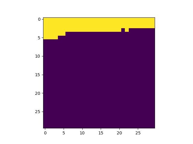
get_field_mask returns an array with non-zeros values
for pixels matching a field:
In [23]: plt.figure()
Out[23]: <Figure size 640x480 with 0 Axes>
In [24]: plt.imshow(fmap.get_field_mask('UDF-06'), vmin=0, vmax=1)
�������������������������������������������Out[24]: <matplotlib.image.AxesImage at 0x7f106d97de48>
In [25]: plt.figure()
Out[25]: <Figure size 640x480 with 0 Axes>
In [26]: plt.imshow(fmap.get_field_mask('UDF-09'), vmin=0, vmax=1)
�������������������������������������������Out[26]: <matplotlib.image.AxesImage at 0x7f106e18bf60>
Reference/API
mpdaf.MUSE Package
Functions
create_psf_cube(shape, fwhm[, beta, wcs, …]) |
Create a PSF cube with FWHM varying along each wavelength plane. |
get_FSF_from_cube_keywords(cube, size) |
Return a cube of FSFs corresponding to the keywords presents in the MUSE data cube primary header (‘FSF***’) |
Classes
FSF([typ]) |
This class offers Field Spread Function (FSF) models for MUSE. |
FieldsMap([filename, nfields]) |
Class to work with the mosaic field map. |
LSF([typ]) |
This class offers Line Spread Function models for MUSE. |
Slicer |
Convert slice number between the various numbering schemes. |