MUSE specific tools (mpdaf.MUSE)
Python interface for MUSE slicer numbering scheme
The Slicer class contains a set of static methods to convert
a slice number between the various numbering schemes. The definition of the
various numbering schemes and the conversion table can be found in the “Global
Positioning System” document (VLT-TRE-MUSE-14670-0657).
All the methods are static and thus there is no need to instantiate an object to use this class.
For example, we convert slice number 4 in CCD numbering to SKY numbering:
In [1]: from mpdaf.MUSE import Slicer

In [2]: Slicer.ccd2sky(4)
Out[2]: 10
Now we convert slice number 12 of stack 3 in OPTICAL numbering to CCD numbering:
In [3]: Slicer.optical2sky((2, 12))
Out[3]: 25
MUSE LSF models
Warning
LSF class is currently under development
Only one model of LSF (Line Spread Function) is currently available.
LSF qsim_v1
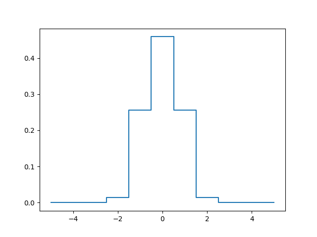
This is a simple model where the LSF is supposed to be constant over the filed of view. It uses a simple parametric model of variation with wavelength.
The model is a convolution of a step function with a Gaussian. The resulting function is then sample by the pixel size:
LSF = T(y2+dy/2) - T(y2-dy/2) - T(y1+dy/2) + T(y1-dy/2)

T(x) = exp(-x**2/2) + sqrt(2*pi)*x*erf(x/sqrt(2))/2

y1 = (y-h/2) / sigma

y2 = (y+h/2) / sigma
The slit width is assumed to be constant (h = 2.09 pixels). The Gaussian sigma parameter is a polynomial approximation of order 3 with wavelength:
c = [-0.09876662, 0.44410609, -0.03166038, 0.46285363]

sigma(x) = c[3] + c[2]*x + c[1]*x**2 + c[0]*x**3
To use it, create a LSF object with attribute ‘typ’ equal to
‘qsim_v1’:
In [4]: from mpdaf.MUSE import LSF

In [5]: lsf = LSF(typ='qsim_v1')
Then get the LSF array by using get_LSF:
In [6]: lsf_6000 = lsf.get_LSF(lbda=6000, step=1.25, size=11)

In [7]: import matplotlib.pyplot as plt

In [8]: import numpy as np

In [9]: plt.plot(np.arange(-5,6), lsf_6000, drawstyle='steps-mid')
Out[9]: [<matplotlib.lines.Line2D at 0x7a86afe6f4d0>]
MUSE FSF models
Warning
FSF class is currently under development
Two models of FSF (Field Spread Function) are currently available:
OldMoffatModel(model='MOFFAT1'): the old model with a fixed beta [DEPRECATED].MoffatModel2(model=2): a circular MOFFAT with polynomials for beta and FWHM.
Example with MoffatModel2
The MUSE FSF is modelled as a Circular Moffat function with a FWHM and beta parameter which varies with the wavelength according to:
\(FWHM = p_0 \times l^n + p_1 \times l^{n-1} + p_n\)
\(\beta = k_0 \times l^m + k_1 \times l^{m-1} + k_m\)
\(l = (\lambda - \lambda_1) / (\lambda_2 - \lambda_1) - 0.5\)
With:
\(p_i\) polynomial coefficient for FWHM polynomial approximation
n FWHM polynomial degre
\(k_i\) polynomial coefficient for beta polynomial approximation
m beta polynomial degre
\(\lambda_1\),:math:
lambda_2reference wavelength for normalisation
We create the FSFModel object like this:
In [10]: from mpdaf.MUSE import FSFModel, MoffatModel2

In [11]: fsf = MoffatModel2(fwhm_pol=[-0.2, 0.7], beta_pol=[2.8], lbrange=[4800,9300], pixstep=0.2)

In [12]: fsf.info()
[INFO] Wavelength range: 4800-9300
[INFO] FWHM Poly: [-0.2, 0.7]
[INFO] FWHM (arcsec): 0.80-0.60
[INFO] Beta Poly: [2.8]
[INFO] Beta values: 2.80-2.80
There are various way to create a fsf model, by fitting a point source or by using the external
PSF reconstruction module muse_psfrec.
Using a star in the field of view
from mpdaf.obj import cube
cube = Cube('DATACUBE.fits')
ra,dec = (53.1583804, -27.7949048)
fsf = MoffatModel2.from_starfit(cube, (dec,ra), fwhmdeg=3, betadeg=2)
[INFO] FSF from star fit at Ra: 53.15838 Dec: -27.79491 Size 5.1 Nslice 20 FWHM poly deg 3 BETA poly deg 2
[debug] getting 20 images around object ra:-27.794905 dec:53.158380
[debug] -- first fit on white light image
[DEBUG] RA: 53.15837 DEC: -27.79492 FWHM 0.66 BETA 2.39 PEAK 276.5 BACK 0.2
[DEBUG] -- Second fit on all images
[DEBUG] 1 RA: 53.15837 DEC: -27.79491 FWHM 0.75 BETA 2.42 PEAK 174.6 BACK 0.1
[DEBUG] 2 RA: 53.15837 DEC: -27.79491 FWHM 0.75 BETA 2.45 PEAK 151.2 BACK 0.1
[DEBUG] ......
[DEBUG] 20 RA: 53.15837 DEC: -27.79493 FWHM 0.60 BETA 2.49 PEAK 293.2 BACK 0.2
[DEBUG] -- Third fit on all images
[DEBUG] -- Polynomial fit of BETA(lbda)
[DEBUG] BETA poly [ 0.07567152 -0.03087214  2.43062733]
[DEBUG] RA: 53.15837 DEC: -27.79491 FWHM 0.75 BETA 2.47 PEAK 174.0 BACK 0.1
[DEBUG] RA: 53.15837 DEC: -27.79491 FWHM 0.75 BETA 2.46 PEAK 151.1 BACK 0.1
[DEBUG] ......
[DEBUG] RA: 53.15837 DEC: -27.79493 FWHM 0.60 BETA 2.44 PEAK 294.2 BACK 0.2
[DEBUG] -- Polynomial fit of FWHM(lbda)
[DEBUG] FWHM poly [ 0.22042019  0.02317024 -0.21365627  0.66766788]
[DEBUG] -- return FSF model
The fsf.fit dictionary can be used to check the fit quality:
fig,ax = plt.subplots(1,2)
ax[0].plot(fsf.fit['wave'], fsf.fit['fwhmfit'], 'ok')
ax[0].plot(fsf.fit['wave'], fsf.fit['fwhmpol'], '-r')
ax[1].plot(fsf.fit['wave'], fsf.fit['betafit'], 'ok')
ax[1].plot(fsf.fit['wave'], fsf.fit['betapol'], '-r')
ax[1].set_ylim(2,3)

Using psfrec
If the MUSE observations have been done in GLAO WFM mode, then one can get a fsf model from the AO telemetry information saved in the raw data.
Warning
The psfrec module must be installed. Check https://muse-psfr.readthedocs.io for information.
fsf = MoffatModel2.from_psfrec('MUSE.2018-09-11T05:44:14.890.fits')
[DEBUG] Computing PSF from Sparta data file MUSE.2018-09-11T05:44:14.890.fits
[INFO] Processing SPARTA table with 13 values, njobs=-1 ...
[INFO] 6/13 : Using only 3 values out of 4 after outliers rejection
[INFO] Compute PSF with seeing=0.69 GL=0.64 L0=18.74
[INFO] Compute PSF with seeing=0.58 GL=0.48 L0=14.40
[INFO] Using three lasers mode
[INFO] Compute PSF with seeing=0.58 GL=0.49 L0=16.65
......
[INFO] Compute PSF with seeing=0.69 GL=0.46 L0=15.24
[INFO] Compute PSF with seeing=0.67 GL=0.56 L0=15.86
[DEBUG] 01: Seeing 0.69,0.69,0.70,0.69 GL 0.64,0.65,0.64,0.63 L0 18.34,19.04,17.48,20.07
[DEBUG] 02: Seeing 0.66,0.65,0.69,0.67 GL 0.57,0.56,0.56,0.54 L0 14.87,18.44,14.24,15.89
......
[DEBUG] 12: Seeing 0.67,0.67,0.66,0.65 GL 0.55,0.51,0.52,0.48 L0 9.37,11.07,10.19,13.05
[DEBUG] 13: Seeing 0.64,0.65,0.69,0.66 GL 0.57,0.56,0.55,0.53 L0 15.43,16.22,12.61,14.41
[DEBUG] Fitting polynomial on FWHM (lbda) and Beta(lbda)
If the MUSE observations have been done in GLAO WFM mode, then one can get a fsf model from the AO telemetry information saved in the raw data.
Warning
The psfrec module must be installed. Check https://muse-psfr.readthedocs.io for information.
Methods
Various methods allow one to get the FSF array (2D or 3D, as mpdaf Image or Cube) for given wavelengths, or the FWHM in pixel and in arcseconds.
In [13]: lbda = np.array([5000, 9000])
In [14]: fsf.get_fwhm(lbda)
Out[14]: array([0.79111111, 0.61333333])
In [15]: fsf.get_fwhm(lbda, unit='pix')
Out[15]: array([3.95555556, 3.06666667])
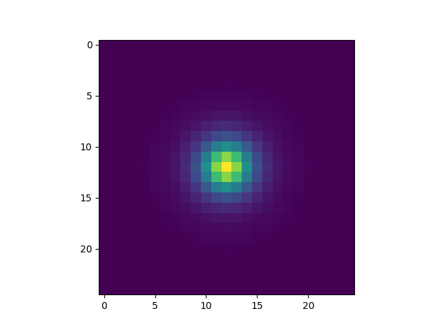
In [16]: im5000 = fsf.get_2darray(lbda[0], shape=(25, 25))
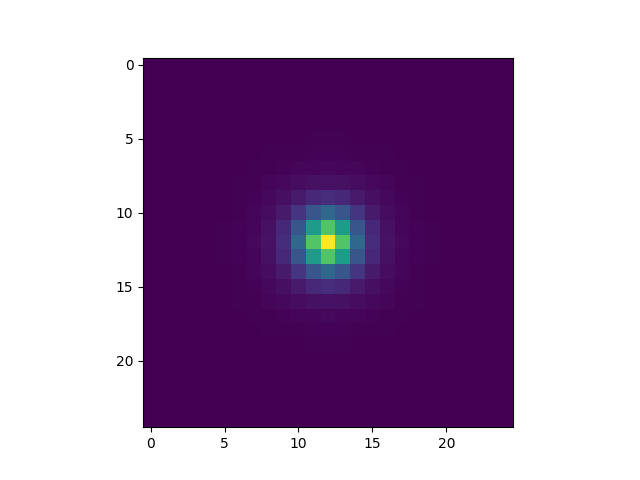
In [17]: fsfcube = fsf.get_3darray(lbda, shape=(25, 25))
In [18]: plt.figure()
Out[18]: <Figure size 640x480 with 0 Axes>
In [19]: plt.imshow(im5000)
Out[19]: <matplotlib.image.AxesImage at 0x7a86ad94da90>
In [20]: plt.figure()
Out[20]: <Figure size 640x480 with 0 Axes>
In [21]: plt.imshow(fsfcube[1])
Out[21]: <matplotlib.image.AxesImage at 0x7a86b02a3d90>
The FSF model can be saved to a FITS header with
mpdaf.MUSE.FSFModel.to_header, and read with mpdaf.MUSE.FSFModel.read.
MUSE mosaic field map
Warning
FieldsMap class is currently under development
FieldsMap reads the possible FIELDMAP extension of the MUSE data
cube.
In [22]: from mpdaf.MUSE import FieldsMap

In [23]: fmap = FieldsMap('sdetect/subcub_mosaic.fits', extname='FIELDMAP')
get_pixel_fields returns a list of fields that cover
a given pixel (y, x):
In [24]: fmap.get_pixel_fields(0,0)
Out[24]: ['UDF-06', 'UDF-09']

In [25]: fmap.get_pixel_fields(20,20)
Out[25]: ['UDF-06']
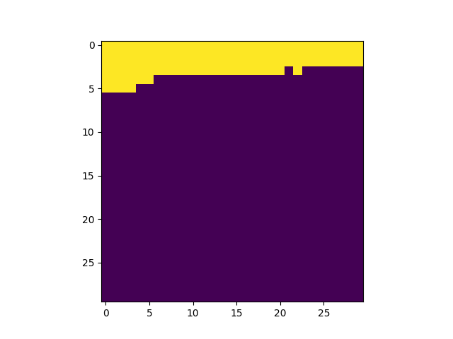
get_field_mask returns an array with non-zeros values
for pixels matching a field:
In [26]: plt.figure()
Out[26]: <Figure size 640x480 with 0 Axes>

In [27]: plt.imshow(fmap.get_field_mask('UDF-06'), vmin=0, vmax=1)
Out[27]: <matplotlib.image.AxesImage at 0x7a86b06402d0>

In [28]: plt.figure()
Out[28]: <Figure size 640x480 with 0 Axes>

In [29]: plt.imshow(fmap.get_field_mask('UDF-09'), vmin=0, vmax=1)
Out[29]: <matplotlib.image.AxesImage at 0x7a86d7b4e990>
Reference/API
mpdaf.MUSE Package
Functions
|
This class offers Field Spread Function (FSF) models for MUSE. |
|
Compute Moffat for a value or array of values of FWHM and beta. |
|
Combine a list of FSF |
|
Create a PSF cube with FWHM varying along each wavelength plane. |
|
Return a cube of FSFs corresponding to the keywords presents in the MUSE data cube primary header ('FSF***') |
Classes
|
Base class for FSF models. |
|
Class to work with the mosaic field map. |
|
This class offers Line Spread Function models for MUSE. |
|
Circular MOFFAT beta=poly(lbda) fwhm=poly(lbda). |
|
Convert slice number between the various numbering schemes. |