Spectrum, Image and Cube format
Attributes
Spectrum, Image and Cube objects all have the following items, where O denotes the name of the object:
Component |
Description |
|---|---|
O.filename |
A FITS filename if the data were loaded from a FITS file |
O.primary_header |
A FITS primary header instance |
O.wcs |
World coordinate spatial information ( |
O.wave |
World coordinate spectral information ( |
O.shape |
An array of the dimensions of the cube |
O.data |
A numpy masked array of pixel values |
O.data_header |
A FITS data header instance |
O.unit |
The physical units of the data values |
O.dtype |
The data-type of the data array (int, float) |
O.var |
An optional numpy masked array of pixel variances |
O.mask |
An array of the masked state of each pixel |
O.ndim |
The number of dimensions in the data, variance and mask arrays |
Masked arrays are arrays that can have missing or invalid entries. The
numpy.ma module
provides a nearly work-alike replacement for numpy that supports data arrays
with masks. See the DataArray documentation for more
details.
When an object is constructed from a MUSE FITS file, O.data will contain the DATA extension,
O.var will contain the STAT extension and O.mask will contain the DQ extension if it exists.
A DQ extension contains the pixel data quality. By default all bad pixels are masked.
But it is possible for the user to create his mask by using the Python interface for euro3D convention.
Indexing
The format of each numpy array follows the indexing used by Python to handle 2D and 3D arrays. For an MPDAF cube C, the pixel in the bottom-lower-left corner is C[0,0,0] and pixel C[k,p,q] refers to the horizontal position q, the vertical position p, and the spectral position k, as follows:
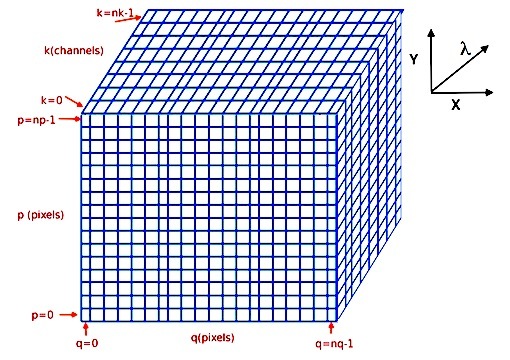
In total, this cube C contains nq pixels in the horizontal direction, np pixels in the vertical direction and nk channels in the spectral direction. In the cube, each numpy masked array has 3 dimensions, array[k,p,q], where k is the spectral axis, and p and q are the spatial axes:
In [1]: from mpdaf.obj import Cube

# data array is read from the file (extension number 0)
In [2]: cube = Cube(filename='sdetect/minicube.fits')

# The 3 dimensions of the cube:
In [3]: cube.shape
Out[3]: (3681, 40, 40)

In [4]: cube.data.shape
Out[4]: (3681, 40, 40)

In [5]: cube.var.shape
Out[5]: (3681, 40, 40)

In [6]: cube.mask.shape
Out[6]: (3681, 40, 40)
Cube[k,p,q] returns the value of Cube.data[k,p,q]:
In [7]: cube[3659, 8, 28]
Out[7]: np.float64(493.9726257324219)
Similarly Cube[k,p,q] = value sets the
value of Cube.data[k,p,q], and Cube[k1:k2,p1:p2,q1:q2] = array sets the corresponding subset of
Cube.data. Finally Cube[k1:k2,p1:p2,q1:q2]
returns a sub-cube, as demonstrated in the following example:
In [8]: cube.info()
[INFO] 3681 x 40 x 40 Cube (sdetect/minicube.fits)
[INFO] .data(3681 x 40 x 40) (1e-20 erg / (Angstrom s cm2)), .var(3681 x 40 x 40)
[INFO] center:(10:27:56.39623411,04:13:25.35875899) size:(8.000",8.000") step:(0.200",0.200") rot:-0.0 deg frame:FK5
[INFO] wavelength: min:4749.89 max:9349.89 step:1.25 Angstrom

In [9]: cube[3000:,10:20,25:40].info()
[INFO] 681 x 10 x 15 Cube (sdetect/minicube.fits)
[INFO] .data(681 x 10 x 15) (1e-20 erg / (Angstrom s cm2)), .var(681 x 10 x 15)
[INFO] center:(10:27:55.39623325,04:13:25.18927284) size:(2.000",3.000") step:(0.200",0.200") rot:-0.0 deg frame:FK5
[INFO] wavelength: min:8499.89 max:9349.89 step:1.25 Angstrom
Likewise, Cube[k,:,:] returns an Image, as
demonstrated below:
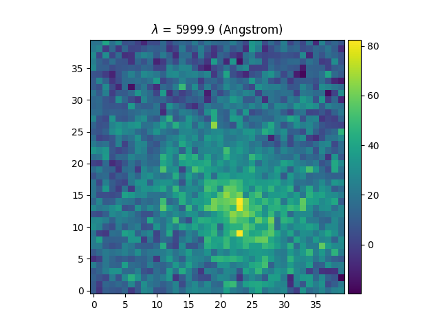
In [10]: ima1 = cube[1000, :, :]
In [11]: plt.figure()
Out[11]: <Figure size 640x480 with 0 Axes>
In [12]: ima1.plot(colorbar='v', title = r'$\lambda$ = %.1f (%s)' %(cube.wave.coord(1000), cube.wave.unit))
Out[12]: <matplotlib.image.AxesImage at 0x7a86b0d5dd10>
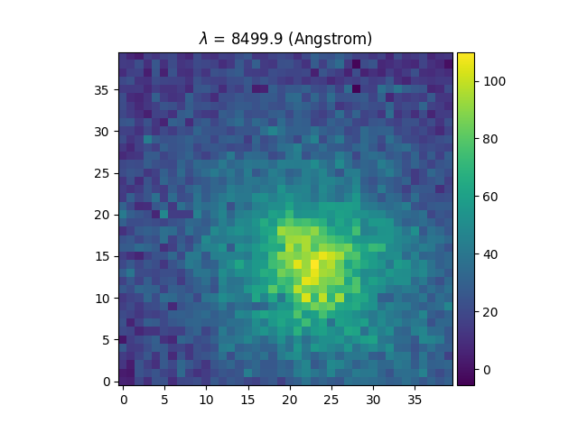
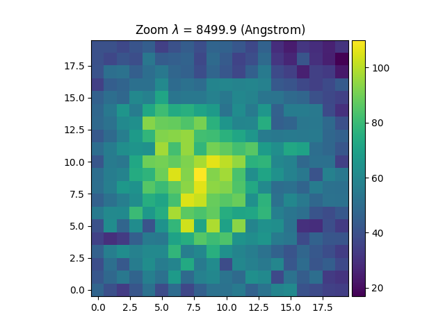
In [13]: ima2 = cube[3000, :, :]
In [14]: plt.figure()
Out[14]: <Figure size 640x480 with 0 Axes>
In [15]: ima2.plot(colorbar='v', title = r'$\lambda$ = %.1f (%s)' %(cube.wave.coord(3000), cube.wave.unit))
Out[15]: <matplotlib.image.AxesImage at 0x7a86b02a0b90>
In [16]: plt.figure()
Out[16]: <Figure size 640x480 with 0 Axes>
In [17]: ima2[5:25, 15:35].plot(colorbar='v',title = r'Zoom $\lambda$ = %.1f (%s)' %(cube.wave.coord(3000), cube.wave.unit))
Out[17]: <matplotlib.image.AxesImage at 0x7a86b0f00050>
In the Image objects extracted from the cube, Image[p1:p2,q1:q2] returns a sub-image, Image[p,q] returns the value of pixel (p,q), Image[p,q] =
value sets value in Image.data[p,q], and
Image[p1:p2,q1:q2] = array sets the
corresponding part of Image.data.
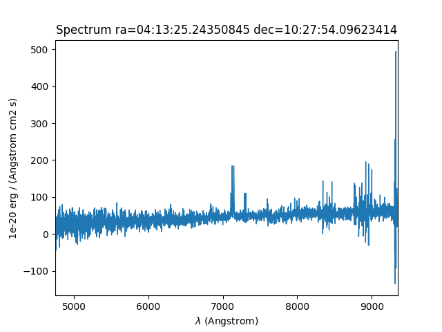
Finally, Cube[:,p,q] returns a Spectrum:
In [18]: spe = cube[:, 8, 28]
In [19]: import astropy.units as u
In [20]: from mpdaf.obj import deg2sexa
In [21]: coord_sky = cube.wcs.pix2sky([8, 28], unit=u.deg)
In [22]: dec, ra = deg2sexa(coord_sky)[0]
In [23]: plt.figure()
Out[23]: <Figure size 640x480 with 0 Axes>
In [24]: spe.plot(title = 'Spectrum ra=%s dec=%s' %(ra, dec))
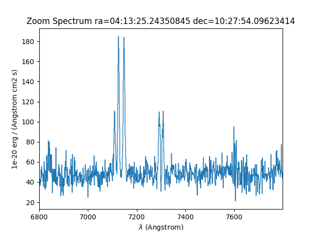
In [25]: plt.figure()
Out[25]: <Figure size 640x480 with 0 Axes>
In [26]: spe[1640:2440].plot(title = 'Zoom Spectrum ra=%s dec=%s' %(ra, dec))
Getters and setters
Cube.get_step, Image.get_step and Spectrum.get_step return the world-coordinate separations between pixels along each axis of a cube, image, or spectrum, respectively:
In [27]: cube.get_step(unit_wave=u.nm, unit_wcs=u.deg)
Out[27]: array([1.25000000e-01, 5.55555556e-05, 5.55555556e-05])

In [28]: ima1.get_step(unit=u.deg)
Out[28]: array([5.55555556e-05, 5.55555556e-05])

In [29]: spe.get_step(unit=u.angstrom)
Out[29]: np.float64(1.25)
Cube.get_range returns the range of wavelengths,
declinations and right ascensions in a cube. Similarly, Image.get_range returns the range of declinations and right
ascensions in an image, and Spectrum.get_range
returns the range of wavelengths in a spectrum, as demonstrated below:
In [30]: cube.get_range(unit_wave=u.nm, unit_wcs=u.deg)
Out[30]:
array([474.9890625 ,  10.46458228,  63.35455983, 934.9890625 ,
        10.46674895,  63.35676316])

In [31]: ima1.get_range(unit=u.deg)
Out[31]: array([10.46458228, 63.35455983, 10.46674895, 63.35676316])

In [32]: spe.get_range(unit=u.angstrom)
Out[32]: array([4749.890625, 9349.890625])
The get_start and get_end methods of cube, image and spectrum objects, return
the world-coordinate values of the first and last pixels of each axis:
In [33]: print(cube.get_start(unit_wave=u.nm, unit_wcs=u.deg), cube.get_end(unit_wave=u.nm, unit_wcs=u.deg))
[474.9890625   10.46458228  63.35676315] [934.9890625   10.46674895  63.35455983]

In [34]: print(ima1.get_start(unit=u.deg), ima2.get_end(unit=u.deg))
[10.46458228 63.35676315] [10.46674895 63.35455983]

In [35]: print(spe.get_start(unit=u.angstrom), spe.get_end(unit=u.angstrom))
4749.890625 9349.890625
Note that when the declination axis is rotated away from the vertical axis of
the image, the coordinates returned by get_start
and get_end are not the minimum and maximum
coordinate values within the image, so they differ from the values returned by
get_range.
Cube.get_rot and Image.get_rot return the rotation angle of the declination axis to
the vertical axis of the images within these objects:
In [36]: cube.get_rot(unit=u.deg)
Out[36]: np.float64(-0.0)

In [37]: ima1.get_rot(unit=u.rad)
Out[37]: np.float64(-0.0)
Updated flux and variance values can be assigned directly to the O.data and
O.var attributes, respectively. Similarly, elements of the data can be
masked or unmasked by assigning True or False values to the corresponding
elements of the O.mask attribute. Changes to the spatial world coordinates
must be performed using the set_wcs method:
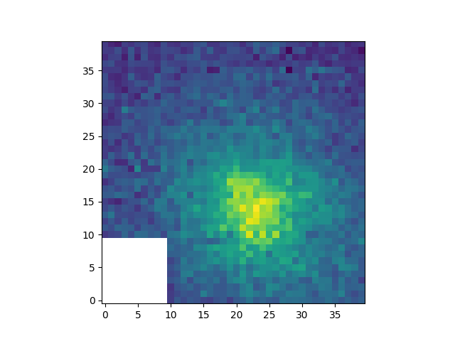
In [38]: ima2.data[0:10,0:10] = 0

In [39]: ima2.mask[0:10,0:10] = True

In [40]: plt.figure()
Out[40]: <Figure size 640x480 with 0 Axes>

In [41]: ima2.plot()
Out[41]: <matplotlib.image.AxesImage at 0x7a86b055a5d0>