Spectrum object
Spectrum objects contain a 1D data array of flux values, and a WaveCoord object that describes the wavelength scale of the
spectrum. Optionally, an array of variances can also be provided to give the
statistical uncertainties of the fluxes. These can be used for weighting the
flux values and for computing the uncertainties of least-squares fits and other
calculations. Finally a mask array is provided for indicating bad pixels.
The fluxes and their variances are stored in numpy masked arrays, so virtually all numpy and scipy functions can be applied to them.
Preliminary imports:
In [1]: import numpy as np

In [2]: import matplotlib.pyplot as plt

In [3]: import astropy.units as u

In [4]: from mpdaf.obj import Spectrum, WaveCoord
Spectrum Creation
There are two common ways to obtain a Spectrum object:
A spectrum can be created from a user-provided array of the flux values at each wavelength of the spectrum, or from both an array of flux values and a corresponding array of variances. These arrays can be simple numpy arrays, or they can be numpy masked arrays in which bad pixels have been masked.
In [5]: wave1 = WaveCoord(cdelt=1.25, crval=4000.0, cunit= u.angstrom)

# numpy data array
In [6]: MyData = np.ones(4000)

# numpy variance array
In [7]: MyVariance=np.ones(4000)

# spectrum filled with MyData
In [8]: spe = Spectrum(wave=wave1, data=MyData)

In [9]: spe.info()
[INFO] 4000 Spectrum (no name)
[INFO] .data(4000) (no unit), no noise
[INFO] wavelength: min:4000.00 max:8998.75 step:1.25 Angstrom

# spectrum filled with MyData and MyVariance
In [10]: spe = Spectrum(wave=wave1, data=MyData, var=MyVariance)

In [11]: spe.info()
[INFO] 4000 Spectrum (no name)
[INFO] .data(4000) (no unit), .var(4000)
[INFO] wavelength: min:4000.00 max:8998.75 step:1.25 Angstrom
Alternatively, a spectrum can be read from a FITS file. In this case the flux and variance values are read from specific extensions:
# data array is read from the file (extension number 0)
In [12]: spe = Spectrum(filename='obj/Spectrum_Variance.fits', ext=0)

In [13]: spe.info()
[INFO] 4096 Spectrum (obj/Spectrum_Variance.fits)
[INFO] .data(4096) (erg / (A s cm2)), no noise
[INFO] wavelength: min:4602.60 max:7184.29 step:0.63 Angstrom

# data and variance arrays read from the file (extension numbers 1 and 2)
In [14]: spe = Spectrum(filename='obj/Spectrum_Variance.fits', ext=[0, 1])

In [15]: spe.info()
[INFO] 4096 Spectrum (obj/Spectrum_Variance.fits)
[INFO] .data(4096) (erg / (A s cm2)), .var(4096)
[INFO] wavelength: min:4602.60 max:7184.29 step:0.63 Angstrom
By default, if a FITS file has more than one extension, then it is expected to have a ‘DATA’ extension that contains the pixel data, and possibly a ‘STAT’ extension that contains the corresponding variances. If the file doesn’t contain extensions of these names, the “ext=” keyword can be used to indicate the appropriate extension or extensions, as shown in the example above.
The WaveCoord object of a spectrum describes the
wavelength scale of the spectrum. When a spectrum is read from a FITS file, this
is automatically generated based on FITS header keywords. Alternatively, when a
spectrum is extracted from a cube or another spectrum, the wavelength object is
derived from the wavelength object of the original object. In the first example
on this page, the wavelength scale of the spectrum increases linearly with array
index, k. The wavelength of the first pixel (k=0) is 4000 Angstrom, and the
subsequent pixels (k=1,2 …) are spaced by 1.25 Angstroms.
Information about a spectrum can be printed using the info method.
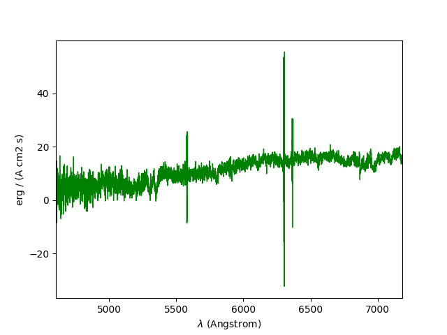
Spectrum objects also have a plot method, which is
based on matplotlib.pyplot.plot
and accepts all matplotlib arguments:
In [16]: plt.figure()
Out[16]: <Figure size 640x480 with 0 Axes>

In [17]: spe.plot(color='g')
This spectrum could also be plotted with a logarithmic scale on the y-axis
(by using log_plot in place of plot).
Spectrum masking and interpolation
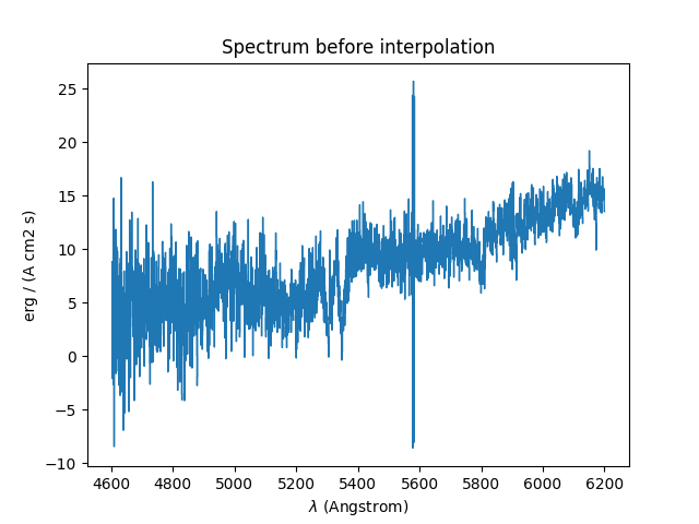
This section demonstrates how one can mask a sky line in a spectrum, and replace it with a linear or spline interpolation over the resulting gap.
The original spectrum and its variance is first loaded:
In [18]: spvar = Spectrum('obj/Spectrum_Variance.fits',ext=[0,1])
Next the mask_region method is used to mask a
strong sky emission line around 5577 Angstroms:
In [19]: spvar.mask_region(lmin=5575, lmax=5590, unit=u.angstrom)
Then the subspec method is used to select the sub-set of
the spectrum that we are interested in, including the masked region:
In [20]: spvarcut = spvar.subspec(lmin=4000, lmax=6250, unit=u.angstrom)
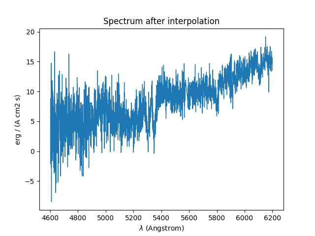
The interp_mask method can then be used to
replace the masked pixels with values that are interpolated from pixels on
either side of the masked region. By default, this method uses linear
interpolation:
In [21]: spvarcut.interp_mask()
However it can also be told to use a spline interpolation:
In [22]: spvarcut.interp_mask(spline=True)
The results of the interpolations are shown below:
In [23]: spvar.unmask()

In [24]: plt.figure()
Out[24]: <Figure size 640x480 with 0 Axes>

In [25]: spvar.plot(lmin=4600, lmax=6200, title='Spectrum before interpolation', unit=u.angstrom)

In [26]: plt.figure()
Out[26]: <Figure size 640x480 with 0 Axes>

In [27]: spvarcut.plot(lmin=4600, lmax=6200, title='Spectrum after interpolation', unit=u.angstrom)
Spectrum rebinning and resampling
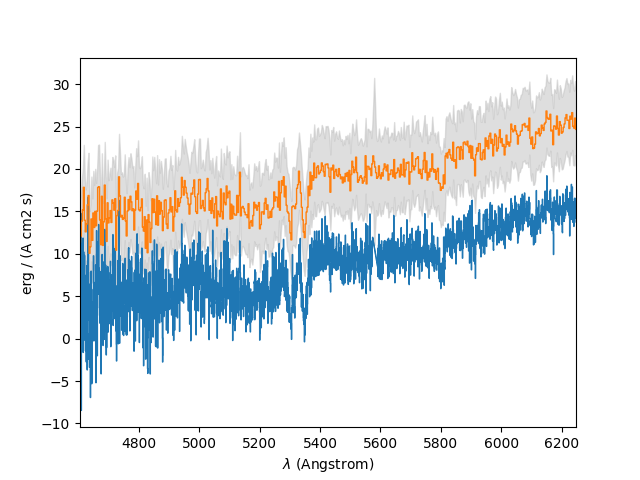
Two methods are provided for resampling spectra. The rebin method reduces the resolution of a spectrum by
integer factors. If the integer factor is n, then the pixels of the new spectrum
are calculated from the mean of n neighboring pixels. If the spectrum has
variances, the variances of the averaged pixels are updated accordingly.
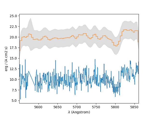
In the example below, the spectrum of the previous section is rebinned to reduce its resolution by a factor of 5. In a plot of the original spectrum, the rebinned spectrum is drawn vertically offset from it by 10. The grey areas above and below the line of the rebinned spectrum indicate the standard deviation computed from the rebinned variances. The standard deviations clearly don’t reflect the actual noise level, but this is because the variances in the FITS file are incorrect.
In [28]: plt.figure()
Out[28]: <Figure size 640x480 with 0 Axes>

In [29]: sprebin1 = spvarcut.rebin(5)

In [30]: spvarcut.plot()

In [31]: (sprebin1 + 10).plot(noise=True)
Whereas the rebin method is restricted to decreasing the resolution by integer
factors, the resample method can resample a
Spectrum to any resolution. The desired pixel size is specified in wavelength
units. At the current time the variances are not updated, but this will be
remedied in the near future.
In [32]: plt.figure()
Out[32]: <Figure size 640x480 with 0 Axes>

In [33]: sp = spvarcut[1500:2000]

# 4.2 Angstroms / pixel
In [34]: sprebin2 = sp.resample(4.2, unit=u.angstrom)

In [35]: sp.plot()

In [36]: (sprebin2 + 10).plot(noise=True)
Continuum and line fitting
Line fitting
In this section, the Hbeta and [OIII] emission lines of a z=0.6758 galaxy are fitted. The spectrum and associated variances are first loaded:
In [37]: specline = Spectrum('obj/Spectrum_lines.fits')
The spectrum around the [OIII] line is then plotted:
In [38]: plt.figure()
Out[38]: <Figure size 640x480 with 0 Axes>

In [39]: specline.plot(lmin=8350, lmax=8420, unit=u.angstrom, title = '[OIII] line')
Next the gauss_fit method is used to perform a
Gaussian fit to the section of the spectrum that contains the line. The fit is
automatically weighted by the variances of the spectrum:
In [40]: OIII = specline.gauss_fit(lmin=8350, lmax=8420, unit=u.angstrom, plot=True)

In [41]: OIII.print_param()
[INFO] Gaussian center = 8390.54 (error:0.15094)
[INFO] Gaussian integrated flux = 633.991 (error:49.0429)
[INFO] Gaussian peak value = 149.684 (error:1.78916)
[INFO] Gaussian fwhm = 3.97902 (error:0.355361)
[INFO] Gaussian continuum = 4.83458
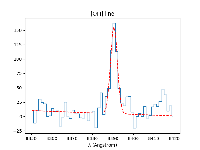
The result of the fit plotted in red over the spectrum.
Next a fit is performed to the fainter Hbeta line, again using the variances to weight the least-squares Gaussian fit:
In [42]: plt.figure()
Out[42]: <Figure size 640x480 with 0 Axes>

In [43]: specline.plot(lmin=8090,lmax=8210, unit=u.angstrom, title = 'Hbeta line')

In [44]: Hbeta = specline.gauss_fit(lmin=8090,lmax=8210, unit=u.angstrom, plot=True)

In [45]: Hbeta.print_param()
[INFO] Gaussian center = 8146.14 (error:0.454373)
[INFO] Gaussian integrated flux = 136.473 (error:44.356)
[INFO] Gaussian peak value = 43.0338 (error:0.917732)
[INFO] Gaussian fwhm = 2.97923 (error:0.904767)
[INFO] Gaussian continuum = 9.23564
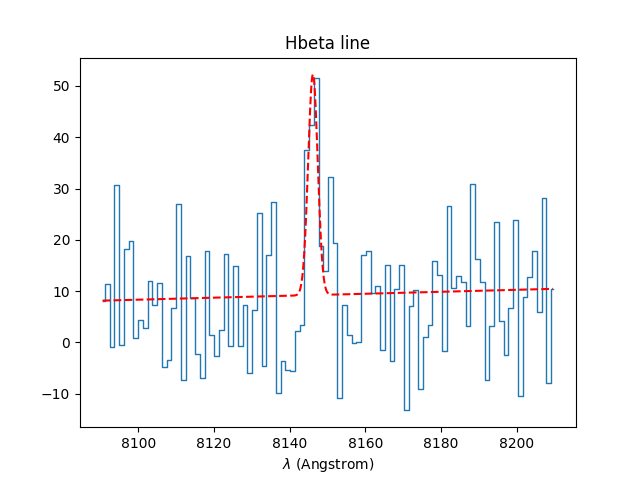
The results from the fit can be retrieved in the returned Gauss1D object. For example the equivalent width of the line can be
estimated as follows:
In [46]: Hbeta.flux/Hbeta.cont
Out[46]: np.float64(14.776784071296156)
If the wavelength of the line is already known, using fix_lpeak=True can
perform an better Gaussian fit on the line by fixing the Gaussian center:
In [47]: plt.figure()
Out[47]: <Figure size 640x480 with 0 Axes>

In [48]: specline.plot(lmin=8090,lmax=8210, unit=u.angstrom, title = 'Hbeta line')

In [49]: Hbeta2 = specline.gauss_fit(lmin=8090,lmax=8210, lpeak=Hbeta.lpeak, unit=u.angstrom, plot=True, fix_lpeak=True)

In [50]: Hbeta2.print_param()
[INFO] Gaussian center = 8146.14 (error:0)
[INFO] Gaussian integrated flux = 136.474 (error:44.1139)
[INFO] Gaussian peak value = 43.0329 (error:1.39697)
[INFO] Gaussian fwhm = 2.97931 (error:0.86632)
[INFO] Gaussian continuum = 9.21934
- In the same way:
gauss_dfitperforms a double Gaussian fit on spectrum.gauss_asymfitperforms an asymetric Gaussian fit on spectrum.
Continuum fitting
The poly_spec method performs a polynomial fit
to a spectrum. This can be used to fit the continuum:
In [51]: plt.figure()
Out[51]: <Figure size 640x480 with 0 Axes>

In [52]: cont = spe.poly_spec(5)

In [53]: spe.plot()

In [54]: cont.plot(color='r')
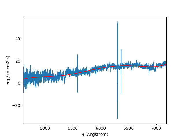
In the plot, the polynomial fit to the continuum is the red line drawn over the spectrum.